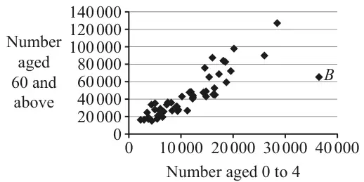
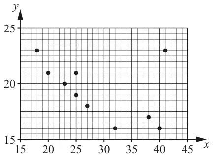
M1: deducing that the first bullet point can be used to: Either set up a correct numerical expression for \(b\) (allow \(\pm\)) implied by \(\pm 0.007\) or \(\pm\dfrac{3.5}{500}\) or write a correct equation from the first bullet point e.g. \(16.5 = a + 2200b\) Allow equivalent use of the first bullet point e.g. \((20 - 3.5k) = a + (1700 + 500k)b\) NB: \((\pm)3.5 = a + 500b\) is M0
A1: \(-0.007\) oe (allow standard form) correct answer scores M1A1.
Mark scheme (b)(ii)
Scheme
Marks
AO
\(20 = a + \text{``}{-0.007}\text{''}(1700)\) or \(20 = a + 1700b\)
M1
2.2a
\(= \underline{31.9}\)
A1
1.1b
(2)
(5 marks)
Notes
M1: using the second bullet point with their value of \(b\) to find \(a\) Either substituting “their \(b\)” into \(20 = a + 1700b\) oe e.g. \(20 - \text{“their }b\text{”} \times 1700\) or writing the correct equation \(20 = a + 1700b\) oe
2. Jasper is investigating the relationship between Daily Mean Pressure and Daily Mean Windspeed (Beaufort conversion) for Perth in 2015 using the data from the large data set.
Treating the large data set for Perth in 2015 as the population, Jasper decides to use all the data available.
(a) Write down the name given to this method of data collection. (1)
All of the Daily Mean Windspeed data for Perth in 2015 are classed as either “Light” or “Moderate”.
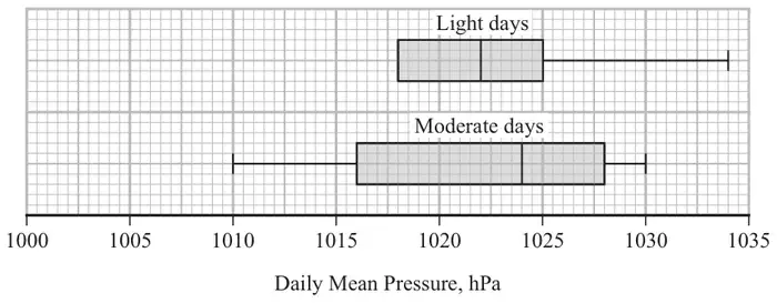
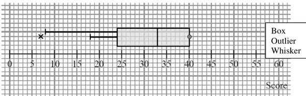
Jasper splits the data for Perth in 2015 into Light days and Moderate days and draws a box plot for each set of data, but omits the lower tail for Light days.
The smallest three values of Daily Mean Pressure for Light days for Perth in 2015 are 1007, 1009 and 1010 hPa.
An outlier in the first quartile is defined as any value more than \(1.5 \times \text{IQR}\) below \(\mathrm{Q}_1\)
(b)
(i) Determine if there are any outliers in the first quartile of Daily Mean Pressure for Light days. (2)
(ii) Hence, complete the box plot of Daily Mean Pressure for Light days. (1)
The box plot for Light days is based on data for 161 days.
(c) Using your knowledge of the large data set, estimate the number of Moderate days with a Daily Mean Pressure of 1028 hPa and higher in the large data set for Perth in 2015. (2)
Mark scheme (a)
Scheme
Marks
AO
Census
B1
1.2
(1)
Notes
B1: cao
Mark scheme (b)(i)
Scheme
Marks
AO
\(1018 - (1025 - 1018) \times 1.5\ (= 1007.5)\)
M1
2.1
\((1007 \lt 1007.5)\) There is one outlier/1007 is an outlier
A1
1.1b
(2)
Notes
M1: finding the correct IQR for “light days” and using it to calculate the lower outlier limit (implied by a correct lower limit 1007.5)
A1: correct outlier limit with correct conclusion Note: 1007 on its own with no supporting working is M0A0.
Mark scheme (b)(ii)
Scheme
Marks
AO
Lower whisker drawn to 1009 and a single outlier at 1007
B1ft
2.2a
Allow lower whisker to end at 1007.5 or 1009
(1)
Notes
B1ft: correct lower whisker drawn to 1009 and single outlier marked at 1007 or correct ft their conclusion to part (b)(i) i.e. if they state there are no outliers, then the lower whisker must be drawn to 1007
Mark scheme (c)
Scheme
Marks
AO
\(184 - 161 = 23\) days with “Moderate” Windspeed
M1
2.4
\(23 \times 0.25 = 5.75\), so 6 days.
A1
2.2b LDS
(2)
(6 marks)
Notes
M1: using knowledge of LDS to find the number of days with “Moderate” Windspeed. Allow use of 180 to 185. Implied by an answer of 5.75 or 19 to 24 from correct knowledge of LDS
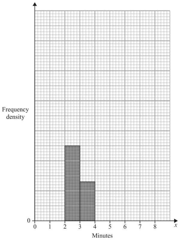
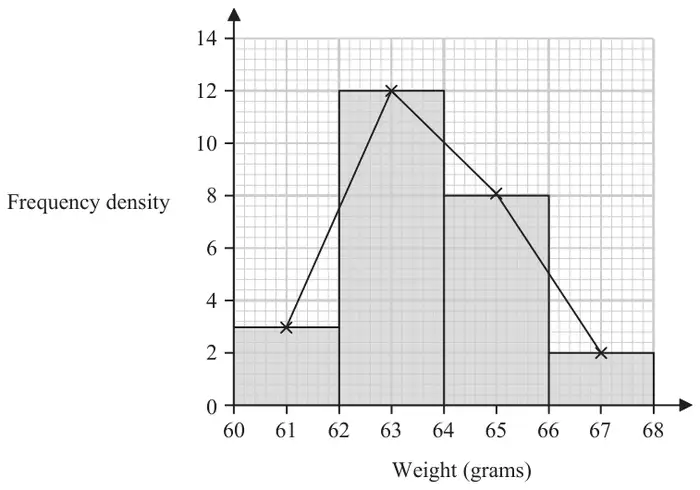
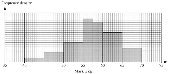
The partially completed table and partially completed histogram below, give information about the time, \(x\) minutes, spent in the queue by each of 112 customers one day.
Time in queue (\(x\) minutes)
Frequency
1–2
64
2–3
3–4
13
4–6
6–8
3
No customer spent less than 1 minute or longer than 8 minutes in the queue.
(a) Complete the table. (2)
(b) Complete the histogram. (2)
Ting decides to model the frequency density for these 112 customers by a curve with equation\[y = \frac{k}{x^2} \qquad 1 \leqslant x \leqslant 8\]where \(k\) is a constant.
(c) Find the value of \(k\) (3)
Mark scheme (a)
Scheme
Marks
AO
[From 3~4 bar and freq in table deduce] fd scale of 1cm = 5
M1
2.2a
2~3 has freq = 25and 4~6 has freq = 112 – (64+13+3 + “25”) = 7
A1
1.1b
(2)
Notes
M1 for deducing a correct fd scale (seen on graph or in text) may be implied 25 or 7 if 25 or 7 found, then ignore their fd scale
A1 for both 25 and 7
Mark scheme (b)
Scheme
Marks
AO
For a bar between 4~6 of height \(\tfrac{\text{``}7\text{''}}{2} = 3.5\) small squares or For a bar between 6~8 of height 1.5 small squares
M1
2.2a
For a fully correct histogram with all 3 bars plotted correctly
A1ft
1.1b
(2)
Notes
Ignore their fd scale in part (b)
M1 for a correct bar over 4~6 follow through their “7” from their table or for a correct bar over 6~8
A1ft for a fully correct histogram (all 3 bars correct height and correct width) allow ft on their 4~6 bar
i.e. \(\left[\dfrac{7}{8}k = 112 \Rightarrow\right]\) \(k =\) 128
A1
1.1b
(3)
(7 marks)
Notes
1st M1 for correct integral expression = 112 (condone missing d\(x\) and ignore limits) or attempt to integrate (\(x^{-2} \to x^{-1}\)) and set area = 112 (ignore limits)
2nd M1 for correct integration and some use of limits of 1 and 8 (condone missing 112) \(\dfrac{7}{8}k = 112\) implies M1M1
2. Keith is studying the variable Daily Mean Wind Direction, in degrees, from the large data set.
Keith summarised the data for Camborne from 1987 into 4 directions \(A\), \(B\), \(C\) and \(D\) representing North, South, East and West in some order.
Direction
\(A\)
\(B\)
\(C\)
\(D\)
Frequency
22
48
56
58
(a) Using your knowledge of the large data set state, giving a reason, which direction \(A\) represents. (1)
The entry for Hurn on 27th September 1987 was 999
(b) State, giving a reason, what Keith should do with this value. (2)
Mark scheme (a)
Scheme
Marks
AO
East Since : The prevailing winds in Camborne/UK are from the South or West or North or East since lowest frequency or Camborne is in South/West (and so wind is less likely to come from East)
B1
2.2b
(1)
Notes
B1 for East and a suitable reason based on: general winds in UK / Camborne allow East and Camborne indicated on a sketch of map contradictory comment e.g. ‘Camborne is in the North, so wind is less likely to come from the East’ is B0
Mark scheme (b)
Scheme
Marks
AO
e.g. ‘wind direction should be in the range 0 to 360’
M1
2.4/1.2
e.g. ‘so he should ignore/remove the value’
A1
1.1b
(2)
(3 marks)
Notes
M1 for giving a reason which correctly uses 360 for reason allow e.g. ‘only goes up to 360’ also condone ‘10 to 360’ this mark may be implied by e.g. ‘subtract 720’
A1 for stating appropriate action to take provided M1 clearly scored ignore o.e. or remove o.e. allow e.g. ‘reject’ , ‘discard’ , etc. must be suggesting what to do with the value, not just stating that it is an anomaly allow change it to 279
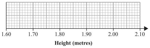
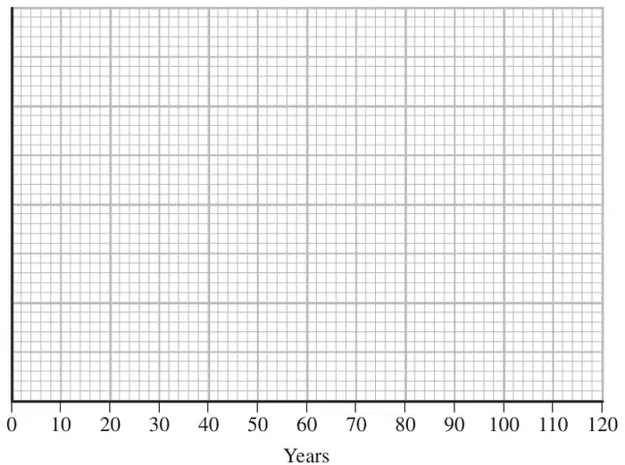
25% of the players’ heights are below the height of a player whose height is 1.81 m
Draw a box and whisker plot to represent this information on the grid below. (4)
Mark scheme
Scheme
Marks
AO
B1 B1ft B1 B1ft
2.2a 1.1b 2.2a 1.1b
(4 marks)
Notes
1st B1 for a box with 2 whiskers (one at each end) with median at 1.85 and lower quartile at 1.81 do not allow median = upper quartile [=1.85]
2nd B1ft for 1.92 plotted as the upper quartile (must be right hand end of box) or for plotting an IQR = 0.11, i.e. their upper quartile at “1.81” + 0.11
3rd B1 for lower whisker ending at 1.72 must be attached to whisker
4th B1ft for upper whisker ending 2.0 must be attached to whisker or for plotting a range of 0.28 i.e. their upper whisker ending at “1.72” + 0.28 for ft condone maximum and/or minimum plotted as outliers by * or ×
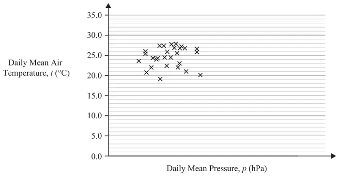
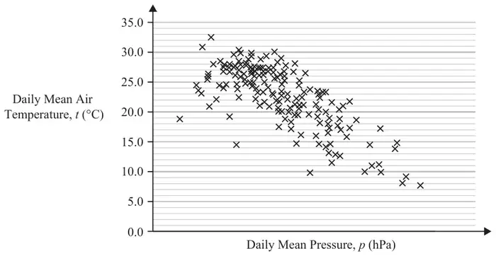
2. Fred and Nadine are investigating whether there is a linear relationship between Daily Mean Pressure, \(p\) hPa, and Daily Mean Air Temperature, \(t\ ^\circ\mathrm{C}\), in Beijing using the 2015 data from the large data set.
Fred randomly selects one month from the data set and draws the scatter diagram in Figure 1 using the data from that month.
The scale has been left off the horizontal axis.
Figure 1
(a) Describe the correlation shown in Figure 1. (1)
Nadine chooses to use all of the data for Beijing from 2015 and draws the scatter diagram in Figure 2.
She uses the same scales as Fred.
Figure 2
(b) Explain, in context, what Nadine can infer about the relationship between \(p\) and \(t\) using the information shown in Figure 2. (1)
(c) Using your knowledge of the large data set, state a value of \(p\) for which interpolation can be used with Figure 2 to predict a value of \(t\). (1)
(d) Using your knowledge of the large data set, explain why it is not meaningful to look for a linear relationship between Daily Mean Wind Speed (Beaufort Conversion) and Daily Mean Air Temperature in Beijing in 2015. (1)
Mark scheme (a)
Scheme
Marks
AO
No (correlation)/weak (correlation)
B1
1.1b
(1)
Notes
B1: correct description of correlation (oe) (ignore reference to positive/negative) condone neutral
Mark scheme (b)
Scheme
Marks
AO
(Negative correlation…) As p(ressure) increases, t(emperature) decreases.
B1
2.2b
(1)
Notes
B1: correct inference, allow equivalent statements. Negative correlation on its own is B0. Inversely proportional on its own is B0.
Mark scheme (c)
Scheme
Marks
AO
990 to 1040 (hPa)
B1
3.4 LDS
(1)
Notes
B1: an answer in the range 990 to 1040 inclusive (ignore units)
Mark scheme (d)
Scheme
Marks
AO
Daily mean wind speed (Beaufort) is a qualitative variable.
B1
2.4 LDS
(1)
(4 marks)
Notes
B1: correct explanation that in the LDS, wind speed (Beaufort) is qualitative/not quantitative Allow e.g. ‘categorical’, e.g. ‘given in words’, e.g. ‘wind speed is (always) light’ Do not allow ‘not continuous’ on its own.
M1: at least 3 correct products seen (oe) Allow any 3 from 366, 1512, 1040, 268
A1*cso: correct expression for mean (which may be seen in stages) and given answer. \(\frac{3186}{50} = 63.72\) on its own is M0A0, but \(\frac{3186}{50} = 63.72\) following all 4 correct products seen can score M1A1
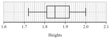
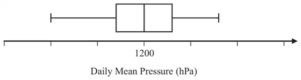
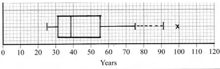
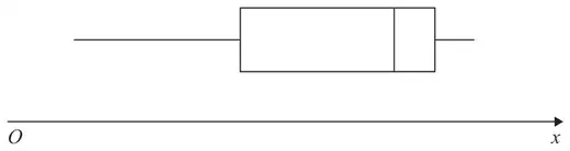
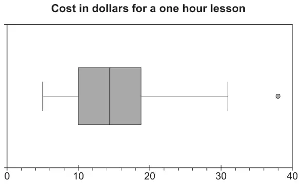
4. Jiang is studying the variable Daily Mean Pressure from the large data set.
He drew the following box and whisker plot for these data for one of the months for one location using a linear scale but
he failed to label all the values on the scale
he gave an incorrect value for the median
Using your knowledge of the large data set, suggest a suitable value for
(a) the median, (1)
(b) the range. (1)
(You are not expected to have memorised values from the large data set. The question is simply looking for sensible answers.)
Mark scheme (a)
Scheme
Marks
AO
Accept 990 to 1030 inclusive
B1
1.1b
(1)
Notes
B1 (Median pressures usually around 1000~1020) [LDS mark]
Mark scheme (b)
Scheme
Marks
AO
Any range between 10 and 50 inclusive
B1
1.1b
(1)
(2 marks)
Notes
B1 Any answer in this range [LDS mark] Allow answers in the form \(a \sim b\) where \(|b - a|\) is between 10 and 50 Also allow the case where both \(a\) and \(b\) are in [10, 50]
1st M1 for an attempt to form frequency table (at least 1st 4 rows and freq or cum freq seen must have the frequency of 75 correct and can condone one error/omission in 15, 35, 55) Frequencies or cum freq may be seen on bars of the histogram
1st A1 for identifying class, freq and cum freq (i.e. highlighted values from the table, shown in bold above) or sight of 3.5-4.5, freq of 55 and “128” – 125 or 180 – “128” or diagram with 125, “128”, 180, 3.5 & 4.5 May be implied by values in 2nd M1 expression
2nd M1 for a correct calculation for \(Q_2\) (condone error in end point e.g. 3.45 or 3.49 etc) Can ft their “125” (provided > 100) and their “55” Allow use of \((n + 1)\), usually see 128.5 – … leading to 3.5636… or awrt 3.56
2nd A1 awrt 3.55 but 3.555 is fine (allow 3.56 if \((n + 1)\) being used …need sight of \(\frac{257}{2}\) etc) Correct answer with no incorrect working scores 4/4
Mark scheme (b)
Scheme
Marks
AO
Need area under curve to be 256 so \(\displaystyle\int_{(0)}^{(8)} kx(8 - x)\,\mathrm{d}x = 256\)
1st M1 for identifying the need to find the area under the curve by integrating
2nd M1 for correct integration and \(= 256\) (condone missing limits)
A1 for \(k = 3\) [May see use of calculator for the integration so score 2nd M1A1 together]
Mark scheme (c)
Scheme
Marks
AO
[By symmetry median = ] 4
B1
2.2a
(1)
(8 marks)
Notes
NB The answer to part (c) may be written within the question.
B1 for 4 (Independent of their value of \(k\) but must be their “\(x\)” value) NB when \(k = 0.25\) and \(x = 4\) gives \(y = 4\) so must be clear they intend median = 4 The statement in part (c) “\(k = 4\)” is B0
1. The relationship between two variables \(p\) and \(t\) is modelled by the regression line with equation
\[p = 22 - 1.1\,t\]
The model is based on observations of the independent variable, \(t\), between 1 and 10
(a) Describe the correlation between \(p\) and \(t\) implied by this model. (1)
Given that \(p\) is measured in centimetres and \(t\) is measured in days,
(b) state the units of the gradient of the regression line. (1)
Using the model,
(c) calculate the change in \(p\) over a 3-day period. (2)
Tisam uses this model to estimate the value of \(p\) when \(t = 19\)
(d) Comment, giving a reason, on the reliability of this estimate. (1)
Mark scheme (a)
Scheme
Marks
AO
Negative (since gradient of regression line is negative)
B1
1.2
(1)
Notes
Answers may be written within the question.
B1 for stating “negative”. Allow a correct interpretation e.g. as \(t\) increases then \(p\) decreases (o.e.) [ignore any values] B0 for contradictory statements e.g. “negative correlation since as \(t\) increases \(p\) increases”
Mark scheme (b)
Scheme
Marks
AO
cm/day (o.e. e.g. cm day−1)
B1
2.2a
(1)
Notes
B1 for a correct description of the units (allow fraction, /, or “per” and allow “d” for “day”)
Mark scheme (c)
Scheme
Marks
AO
\(3 \times [\pm]1.1\)
M1
3.4
= decrease of 3.3 [cm]
A1
1.1b
(2)
Notes
M1 for attempt at a calculation (allow use of \(t = x\) and \(t = x + 3\) followed by subtraction that should lead to 3.3)
A1 for correct description must include word “decrease” (o.e.) and value “3.3” Just seeing: \(22 - 1.1 \times 3 = 18.7\) is M0A0 BUT going on to subtract 18.7 from 22 scores M1 Reaching 3.3 and stating “decrease” or “reduced” (o.e.) will score the A1 too An answer of \(-3.3\) without a word describing decrease (o.e.) will just score M1A0
Mark scheme (d)
Scheme
Marks
AO
19 is (well) outside the range [1, 10] or involves extrapolation (o.e.) so (possibly) unreliable/ inaccurate (o.e.)
B1
2.4
(1)
(5 marks)
Notes
B1 for stating “unreliable” (o.e.) and giving a suitable reason based on idea of extrapolation Must have both statement about reliability and suitable reason e.g. \(t = 19\) is too big or (Model is based on) \(t\) between 1 and 10 (only) [since this implies \(t = 19\) is too big] Allow e.g. (model) “may not work” because of “extrapolation” Just saying “no” since “extrapolation” is B0 but “unreliable”(o.e.) since “extrapolation” is B1
3. Helen is studying one of the qualitative variables from the large data set for Heathrow from 2015.
She started with the data from 3rd May and then took every 10th reading.
There were only 3 different outcomes with the following frequencies
Outcome
\(A\)
\(B\)
\(C\)
Frequency
16
2
1
(a) State the sampling technique Helen used. (1)
(b) From your knowledge of the large data set
(i) suggest which variable was being studied,
(ii) state the name of outcome \(A\). (2)
George is also studying the same variable from the large data set for Heathrow from 2015. He started with the data from 5th May and then took every 10th reading and obtained the following
Outcome
\(A\)
\(B\)
\(C\)
Frequency
16
1
1
Helen and George decided they should examine all of the data for this variable for Heathrow from 2015 and obtained the following
Outcome
\(A\)
\(B\)
\(C\)
Frequency
155
26
3
(c) State what inference Helen and George could reliably make from their original samples about the outcomes of this variable at Heathrow, for the period covered by the large data set in 2015. (1)
Mark scheme (a)
Scheme
Marks
AO
Systematic (sampling)
B1
1.2
(1)
Notes
B1 for identifying the correct sampling technique Allow slight misspelling e.g. “sysmatic”, “sytmatic” Do NOT allow “systemic”
Mark scheme (b)
Scheme
Marks
AO
(i) [Daily Mean] Wind Speed
B1
2.2a
(ii) Light
B1
1.2
(2)
Notes
(i) B1 for identifying appropriate qualitative variable. {LDS mark} Allow “Wind speed” or “Wind strength” but NOT just “wind” or “wind direction”
(ii) B1 for realising that modal wind speed is “Light” {LDS mark} Allow just “light” or “most light”
NB These two B marks are independent so can score B0B1 for e.g. “rainfall” and “light”
Mark scheme (c)
Scheme
Marks
AO
Variable \(A\) occurs most (around 80~90%) of the time
B1
2.2b
(1)
(4 marks)
Notes
B1 for inferring that frequency of \(A\) can be estimated fairly reliably: {underestimates \(B\) and over estimates \(C\)} e.g. “\(A\) is the most frequent” [can then ignore comments about \(B\) and \(C\)]
(i) This would have no effect as the piece of data would remain in the same class
B1
2.2a
(ii) This would increase the standard deviation as change in mean is small and \(6.4 - 4.6 \approx 3\sigma\) therefore estimate of standard deviation will increase
B1
2.2a
(2)
(7 marks)
Notes
B1: Correct deduction with suitable explanation Allow range for class. Do not allow there is no differences
B1: Correct deduction with suitable explanation. so would increase the standard deviation and a suitable reason. Allow the value is bigger than any others in the table oe
2. Jerry is studying visibility for Camborne using the large data set June 1987.
The table below contains two extracts from the large data set.
It shows the daily maximum relative humidity and the daily mean visibility.
Date
Daily Maximum Relative Humidity
Daily Mean Visibility
Units
%
10/06/1987
90
5300
28/06/1987
100
0
(The units for Daily Mean Visibility are deliberately omitted.)
Given that daily mean visibility is given to the nearest 100,
(a) write down the range of distances in metres that corresponds to the recorded value 0 for the daily mean visibility. (1)
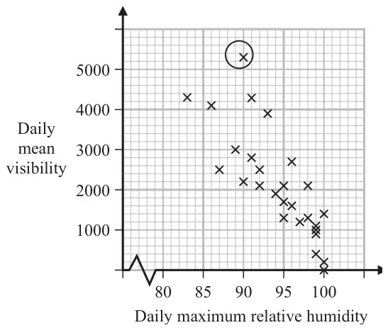
Jerry drew the following scatter diagram, Figure 2, and calculated some statistics using the June 1987 data for Camborne from the large data set.
Figure 2
\(Q_1\)
IQR
Daily mean visibility
1100
1600
Daily maximum relative humidity (%)
92
8
Jerry defines an outlier as a value that is more than 1.5 times the interquartile range above \(Q_3\) or more than 1.5 times the interquartile range below \(Q_1\).
(b) Show that the point circled on the scatter diagram is an outlier for visibility. (2)
(c) Interpret the correlation between the daily mean visibility and the daily maximum relative humidity. (1)
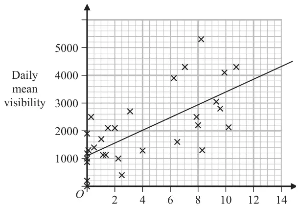
Jerry drew the following scatter diagram, Figure 3, using the June 1987 data for Camborne from the large data set, but forgot to label the \(x\)-axis.
Figure 3
(d) Using your knowledge of the large data set, suggest which variable the \(x\)-axis on this scatter diagram represents. (1)
Mark scheme (a)
Scheme
Marks
AO
0 to 500 m
B1
1.2
(1)
Notes
B1: For realising it is the maximum distance and distance given with correct units. Allow 0 to 50dm or < 500m or < 50dm
Mark scheme (b)
Scheme
Marks
AO
\(1100 + 1600 + 1.5 \times 1600\ [= 5100]\)
M1
2.1
5300 > 5100 therefore outlier
A1
1.1b
(2)
Notes
M1: Attempt to find \(Q_3\) and the upper limit
A1: 5100, if a value for the point is stated it must be above 5100 otherwise it is A0. For a statement comparing and conclusion it is an outlier or it is above \(Q_3 + 1.5\text{IQR}\). Allow accept the point circled is greater than 5100 oe
Mark scheme (c)
Scheme
Marks
AO
As the humidity increases the mean visibility decreases
B1
2.4
(1)
Notes
B1: For a suitable interpretation of a negative correlation mentioning humidity and visibility
Mark scheme (d)
Scheme
Marks
AO
(Hours of) sunshine
B1
2.2b
(1)
(5 marks)
Notes
B1: A correct deduction that the unlabelled variable is the hours of sunshine. Condone missing hours. Do not allow if more than one variable given. Must be quantative variable Not cloud cover since values bigger than 8 Not wind speed since values not integers Not daily mean temperature since mean temperature near to zero are unlikely in June
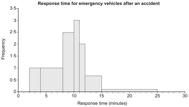
M1: For clear use of frequency density to establish the fd scale and then use the area to find frequency of <11 minutes. Allow maximum of 3 errors in either the heights or widths in total if working shown. They may calculate the area using other size squares. Allow for realising they need to find the total number of squares (88) maximum of 4 errors in either the heights or widths and number < 11 minutes(16) - must have a maximum of 1 error in either the heights or widths (and not use the 78 as part of calulation)
A1: For correct values seen. Allow for 88 and 16
M1: For realising the need to find the total and calculating a percentage. ( with “their 24” as the numerator). Allow \((8 \times 1 + 2 \times 8) \times \text{``}1.5\text{''}\) instead of \(\text{``}24\text{''} + 1 \times 8 \times \text{``}1.5\text{''}\) If working shown can allow maximum of 2 errors in either the heights or widths in the calculation of the total. Allow “their 24” / 132 oe
4. Joshua is investigating the daily total rainfall in Hurn for May to October 2015
Using the information from the large data set, Joshua wishes to calculate the mean of the daily total rainfall in Hurn for May to October 2015
(a) Using your knowledge of the large data set, explain why Joshua needs to clean the data before calculating the mean. (1)
Using the information from the large data set, he produces the grouped frequency table below.
Daily total rainfall (\(r\) mm)
Frequency
Midpoint (\(x\) mm)
\(0 \leqslant r < 0.5\)
121
0.25
\(0.5 \leqslant r < 1.0\)
10
0.75
\(1.0 \leqslant r < 5.0\)
24
3.0
\(5.0 \leqslant r < 10.0\)
12
7.5
\(10.0 \leqslant r < 30.0\)
17
20.0
You may use \(\sum fx = 539.75\) and \(\sum fx^2 = 7704.1875\)
(b) Use linear interpolation to calculate an estimate for the upper quartile of the daily total rainfall. (2)
(c) Calculate an estimate for the standard deviation of the daily total rainfall in Hurn for May to October 2015 (2)
(d)
(i) State the assumption involved with using class midpoints to calculate an estimate of a mean from a grouped frequency table.
(ii) Using your knowledge of the large data set, explain why this assumption does not hold in this case.
(iii) State, giving a reason, whether you would expect the actual mean daily total rainfall in Hurn for May to October 2015 to be larger than, smaller than or the same as an estimate based on the grouped frequency table. (3)
Mark scheme (a)
Scheme
Marks
AO
Tr(ace) (data needs to be converted to numbers before the calculation can be carried out)
B1
2.4
(1)
Notes
B1: Identifying tr(ace) data Ignore comments about n/a, missing data, anomalies, etc.
Mark scheme (b)
Scheme
Marks
AO
\([1+]\,\dfrac{138 - 131}{24} \times 4\)
M1
2.1
\(= 2.1666\ldots\) awrt 2.17
A1
1.1b
(2)
Notes
M1: Correct fraction \(\dfrac{7}{24} \times 4\) allow working down \([5] - \dfrac{155 - 138}{24} \times 4\) allow a correct equation leading to a correct fraction e.g. \(\dfrac{x - 1}{5 - 1} = \dfrac{138 - 131}{155 - 131}\) for M1 Use of \((n + 1)\) with 138.75 allow \(\dfrac{7.75}{24} \times 4\)
(i) Using class midpoints to estimate the mean assumes that the values are uniformly distributed within the class(es).
B1
2.4
(ii) & (iii) This is not the case here as the majority of the data (in the first class) are 0.
B1
2.3
The actual mean is likely to be smaller than the estimate (since the first group has more values at 0 and close to 0)
dB1
2.2b
(3)
(8 marks)
Notes
(d)(i)
B1: Explaining that data assumed to be spread evenly across each class (o.e.) e.g. The midpoint of each class is the mean of each class or all the values in the class are located at the midpoint condone normally distributed within each class
Mark together (ii)&(iii)
B1: Demonstrating an understanding of the LDS that the majority of data values (in the first class) are at 0 or close to 0 (trace).
dB1: (dependent upon 2nd B1) Correct inference based on knowledge of the LDS
SC: If B1 is scored in (i) for ‘The data are spread evenly across each class,’ then in (ii) ‘The data are not evenly distributed in the classes’ scores B1 but in (iii) ‘the actual mean is smaller’ with no further justification scores B0
1. A sixth form college has 84 students in Year 12 and 56 students in Year 13
The head teacher selects a stratified sample of 40 students, stratified by year group.
(a) Describe how this sample could be taken. (3)
The head teacher is investigating the relationship between the amount of sleep, \(s\) hours, that each student had the night before they took an aptitude test and their performance in the test, \(p\) marks. For the sample of 40 students, he finds the equation of the regression line of \(p\) on \(s\) to be\[p = 26.1 + 5.60s\]
(b) With reference to this equation, describe the effect that an extra 0.5 hours of sleep may have, on average, on a student’s performance in the aptitude test. (1)
(c) Describe one limitation of this regression model. (1)
Mark scheme (a)
Scheme
Marks
AO
Label each year group
B1
1.1b
Use random numbers to select a ...
B1
1.1b
Simple random sample of 24 Year 12s and 16 Year 13s.
B1
1.1b
(3)
Notes
B1: for a suitable numbered/labelled/ordered(o.e.) list/database/register(o.e.) for each year group. Condone poor numbering but if just one list, then the Year 12s must be distinguishable from the Year 13s
B1: for use of random numbers/sample/selection to choose students
B1: for 24 Year 12s, and 16 Year 13s
Note: A description of a systematic sample: only allow access to the first mark and therefore may score maximum B1B0B0
Mark scheme (b)
Scheme
Marks
AO
Increase by 2.8 marks
B1
3.4
(1)
Notes
B1: Using the gradient of the regression equation must include increase(o.e.) and 2.8 ‘Increase by approximately 3 marks’ is B0 but isw if 2.8 is seen \(5.6 \div 2\) is not sufficient
Mark scheme (c)
Scheme
Marks
AO
e.g. ‘the best performance is predicted for the students who never wake up’
B1
3.5b
(1)
(5 marks)
Notes
B1: for any suitable limitation of the model e.g. the idea that the longer you sleep the better performance in the test or only valid between 0 and 24 hours (within range of the data) or only applicable to the amount of sleep the night before the test or only takes sleep into consideration/does not include other variables (factors) or cannot score below 26.1 marks on the test or the model might not be linear over the entire range or the model might predict more than the maximum mark
B0: e.g. might not be correlation between \(s\) and \(p\) or individual student performance may vary
4. Helen is studying the daily mean wind speed for Camborne using the large data set from 1987.
The data for one month are summarised in Table 1 below.
Windspeed
n/a
6
7
8
9
11
12
13
14
16
Frequency
13
2
3
2
2
3
1
2
1
2
Table 1
(a) Calculate the mean for these data. (1)
(b) Calculate the standard deviation for these data and state the units. (2)
The means and standard deviations of the daily mean wind speed for the other months from the large data set for Camborne in 1987 are given in Table 2 below. The data are not in month order.
Month
\(A\)
\(B\)
\(C\)
\(D\)
\(E\)
Mean
7.58
8.26
8.57
8.57
11.57
Standard Deviation
2.93
3.89
3.46
3.87
4.64
Table 2
(c) Using your knowledge of the large data set, suggest, giving a reason, which month had a mean of 11.57 (2)
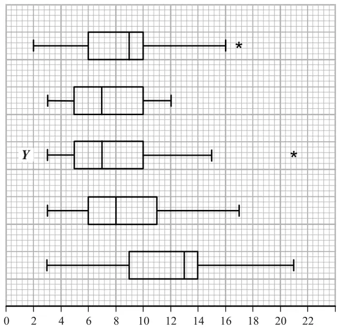
The data for these months are summarised in the box plots below. They are not in month order or the same order as in Table 2.
(d)
(i) State the meaning of the * symbol on some of the box plots.
(ii) Suggest, giving your reasons, which of the months in Table 2 is most likely to be summarised in the box plot marked \(Y\). (3)
Mark scheme (a)
Scheme
Marks
AO
\(\bar{x} = 10.2\,(2222\ldots)\) awrt 10.2
B1
1.1b
(1)
Notes
NB \(\bar{x} = \dfrac{184}{18}\) and \(\sigma_x = \sqrt{\dfrac{2062}{18} - \bar{x}^2}\)
B1 for \(\bar{x} = 10.2\) (allow exact fraction) [This is an LDS mark]
Mark scheme (b)
Scheme
Marks
AO
\(\sigma_x = 3.17\,(20227\ldots)\) awrt 3.17
B1ft
1.1b
Sight of “knots” or “kn” (condone knots/s etc)
B1
1.2
(2)
Notes
NB \(\bar{x} = \dfrac{184}{18}\) and \(\sigma_x = \sqrt{\dfrac{2062}{18} - \bar{x}^2}\)
1st B1ft allow 3.2 from a correct expr’ accept \(s = 3.26(3984\ldots)\) [ft use of n/a] Treating n/a as 0 May see \(n = 31\) or \(\bar{x} = 5.9354\ldots\) which is B0 in (a) but here in (b) it gives \(\sigma_x = 5.59(34\ldots)\) or \(s = 5.6858\ldots\) (awrt 5.69) and scores 1st B1
2nd B1 accept kn accept in (a) or (b) (allow nautical miles/hour) [This is an LDS mark]
Mark scheme (c)
Scheme
Marks
AO
October ….. since
B1
2.2b
it is windier in the autumn or month of the hurricane or latest month in the year
B1
2.4
(2)
Notes
1st B1 choosing October but accept September. [This is an LDS mark]
2nd B1 for stating that (Camborne) is windier in autumn/winter months “because it is winter/autumn/windier/colder in “month” ” Sep \(\leqslant\) "month" \(\leqslant\) Mar scores B1B1 for “month” = Sep or Oct and B0B1 for other months in range
Mark scheme (d)
Scheme
Marks
AO
(i) They represent outliers
B1
1.2
(ii) \(Y\) has low median so expect lowish mean (but outlier so \(\gt 7\)) and \(Y\) has big range/IQR or spread so expect larger st.dev
M1
2.4
Suggests \(B\)
A1
2.2b
(3)
(8 marks)
Notes
(d)(i) B1 for outlier or the idea of an extreme value allow “anomaly”
(ii) M1 for a comment relating to location that mentions both median and mean and a comment relating to spread that mentions both range/IQR and standard deviation and leads to choosing \(B\), \(C\) or \(D\) Choosing \(A\) or \(E\) is M0 Incorrect/false statements score M0 e.g. \(Q_3 = (\text{mean} + \sigma)\) or identify \(Q_2 =\) mean or \(Y\) has small spread
ALTUse of outliers: outlier is \((\text{mean} + 3\sigma)\) \((B = 19.9)\), \((C = 18.95)\), \((D = 20.2)\) Must see at least one of these values and compare to \(Y\)’s outlier [leads to \(D\) or \(B\)]
A1 for suitable inference i.e. \(B\) (accept \(D\) or \(B\) or \(D\)) M1 must be scored
1. A company is introducing a job evaluation scheme. Points (\(x\)) will be awarded to each job based on the qualifications and skills needed and the level of responsibility. Pay (£\(y\)) will then be allocated to each job according to the number of points awarded.
Before the scheme is introduced, a random sample of 8 employees was taken and the linear regression equation of pay on points was \(y = 4.5x - 47\)
(a) Describe the correlation between points and pay. (1)
(b) Give an interpretation of the gradient of this regression line. (1)
(c) Explain why this model might not be appropriate for all jobs in the company. (1)
Mark scheme (a)
Scheme
Marks
AO
Positive (correlation)
B1
1.2
(1)
Notes
B1 for “positive”. Allow an interpretation e.g. “as points increase pay increases” is B1 Read whole answer: contradictory comments such as “positive correlation, as points increase pay decreases” scores B0
Mark scheme (b)
Scheme
Marks
AO
Every extra point gives £4.5(0) more on pay (o.e.)
B1
3.4
(1)
Notes
B1 for any correct comment conveying idea of £s per point and including a correct value; must have idea of rate. Can condone missing £ sign. Accept 4.5 e.g. “every 10 points earns an extra (or increase) of £45” is B1 BUT “every point earns £4.5(0)” is B0 doesn’t have idea of rate
Mark scheme (c)
Scheme
Marks
AO
e.g. For points \(\lt 11\) it would give pay \(\lt 0\) which is ridiculous
B1
2.4
(1)
(3 marks)
Notes
B1 for a suitable comment mentioning “points” or “pay” (o.e. e.g. “amount”) or commenting on “small sample” or “range of points” used to find line
The following examples would score B1 Can say that \(n\) points (for \(n \lt 10.\dot{4}\)) would give negative pay so not suitable Any comment suggesting that some jobs would end up with negative pay Don’t know the range of points used to find the regression line A small sample of size 8 may not be representative to cover all jobs
B0 for a focus on “qualifications” or “hours” worked only
The following examples would score B0 Some jobs require no (or low) skills or qualifications (need negative pay)
2. The following grouped frequency distribution summarises the number of minutes, to the nearest minute, that a random sample of 100 motorists were delayed by roadworks on a stretch of motorway one Monday.
Delay (minutes)
Number of motorists (f)
Delay midpoint (\(x\))
3–6
38
4.5
7–8
25
7.5
9–10
18
9.5
11–15
12
13
16–20
7
18
(You may use \(\sum \mathrm{f}x^2 = 8096.25\))
A histogram has been drawn to represent these data.
The bar representing a delay of (3–6) minutes has a width of 2 cm and a height of 9.5 cm.
(a) Calculate the width and the height of the bar representing a delay of (11–15) minutes. (3)
(b) Use linear interpolation to estimate the median delay. (2)
(c) Calculate an estimate of the mean delay. (2)
(d) Calculate an estimate of the standard deviation of the delays. (2)
One coefficient of skewness is given by \(\dfrac{3(\text{mean} - \text{median})}{\text{standard deviation}}\)
(e) Evaluate this coefficient for the above data, giving your answer to 2 significant figures. (1)
On the following Friday, the coefficient of skewness for the delays on this stretch of motorway was – 0.22
(f) State, giving a reason, how the delays on this stretch of motorway on Friday are different from the delays on Monday. (2)
Mark scheme (a)
Scheme
Marks
(3 – 6 ) mins has width 4 and is 2cm, (11 – 15) mins has width 5 so is 2.5(cm)
B1
(3 – 6) mins has frequency of 38 and area of 19 cm\(^2\) so 2 people(per cm\(^2\))(o.e.) or frequency density \(= \dfrac{38}{4} = 9.5 =\) height
M1
(11 – 15) mins has area of \(2.5 \times h\) cm\(^2\) so \(h = \dfrac{12}{2 \times 2.5} = \)2.4 (cm) allow \(\frac{12}{5}\)
A1
(3)
Notes
B1 for width of 2.5 (cm) allow \(\frac{5}{2}\)
M1 for 2 people per cm\(^2\) or a correct numerical equ’n for \(h\) or their width\(\times\)height = 6
A1 for height of 2.4 (cm) [If just see 2.4 and 2.5 it must be clear which is \(h\) and which \(w\)]
M1 for an attempt at \(\Sigma \mathrm{f}x\) ( i.e. full expression or \(650 \lt \Sigma \mathrm{f}x \lt 950\)) and division by 100 \(\Sigma \mathrm{f}x\) may be in the table.
A1 for 8.115 or awrt 8.12 (allow 8.11) [May be in (d) but must be labelled e.g. \(\bar{x} = \ldots\)]
B1 for a correct expression seen using their values ( \(\sigma\) must be > 0) or awrt 0.47 ~ 0.51
Mark scheme (f)
Scheme
Marks
Skewness for Monday and Friday are different (o.e.)
B1
Suggests more longer delays on Friday (o.e.) [look for diagrams to support this.]
B1
(2)
(12 marks)
Notes
1st B1 for a comment that skewness is different (only commenting on“correlation” is B0) If ans. to (e) > 0 allow B1 for e.g. “skewness on Fri is < 0”[“on Fri” may be implied]
2nd B1 for a comment about length of delay e.g. “more long ones (on Fri.) or “longer delays on Fri.”
M1 For one correct calculation, follow through their 720.
A1 4, 6, 10, 20 only. Must identify which job the values relate to.
Mark scheme (c)
Scheme
Marks
Label all managers 1 – 72 o.e.
B1
Using random numbers in range 1-72 or 0-71 select 4 (managers).
B1
(2)
(6 marks)
Notes
1st B1 Idea of sampling frame or list of managers. Need not give the specific term.
2nd B1 Use of random numbers to select required number of managers. Must mention use of random numbers or some random selection process. If they are describing systematic sampling score B0.
(a) State two reasons why stratified sampling might be a more suitable sampling method than simple random sampling. (2)
(b) State two reasons why stratified sampling might be a more suitable sampling method than quota sampling. (2)
Mark scheme (a)
Scheme
Marks
e.g. Analyse / find estimates for a particular subgroup of the population. Stratified guarantees representation of all groups, srs does not. Observe relationships between subgroups – srs does not guarantee equal or proportionate representation. Rare or extreme cases as part of a small subgroups can be represented proportionately in stratified i.e. stratified represents the structure of the population– srs does not allow this. Stratified typically require large sample size compared to srs due to lower variability within subgroups compared to entire population. Any 2 distinct reasons
B1B1
(2)
Mark scheme (b)
Scheme
Marks
e.g. It (a stratified sample) is not biased as the members are chosen randomly. You can estimate the sampling errors (for a stratified sample) It (a stratrified sample) gives more accurate estimates as it is a random process. A quota sample may be (interviewer / process) biased. It’s not possible to estimate/find the sampling errors for a quota sample (whereas you can for a stratified sample) Any 2 distinct reasons
B1B1
(2)
(4 marks)
Notes
Award B1B1 two correct, B1B0 one correct.
Allow ‘it’ for ‘stratified’.
Do not award marks for vague responses such as ‘cheap’, ‘easy’ ‘quick’ ‘random’ etc.
Mentioning ‘sampling frame’ alone is not sufficient for a mark.
Mentioning ‘non-response are not recorded’ alone is not sufficient for a mark.
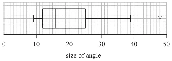
1. Each of 60 students was asked to draw a \(20^\circ\) angle without using a protractor. The size of each angle drawn was measured. The results are summarised in the box plot below.
(a) Find the range for these data. (1)
(b) Find the interquartile range for these data. (1)
The students were then asked to draw a \(70^\circ\) angle. The results are summarised in the table below.
Angle, \(a\), (degrees)
Number of students
\(55 \leqslant a \lt 60\)
6
\(60 \leqslant a \lt 65\)
15
\(65 \leqslant a \lt 70\)
13
\(70 \leqslant a \lt 75\)
11
\(75 \leqslant a \lt 80\)
8
\(80 \leqslant a \lt 85\)
7
(c) Use linear interpolation to estimate the size of the median angle drawn. Give your answer to 1 decimal place. (2)
(d) Show that the lower quartile is \(63^\circ\) (2)
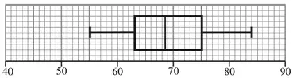
For these data, the upper quartile is \(75^\circ\), the minimum is \(55^\circ\) and the maximum is \(84^\circ\)
An outlier is an observation that falls either more than \(1.5 \times\) (interquartile range) above the upper quartile or more than \(1.5 \times\) (interquartile range) below the lower quartile.
(e)
(i) Show that there are no outliers for these data.
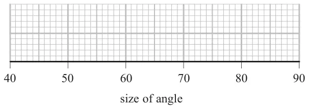
(ii) Draw a box plot for these data on the grid below. (5)
(f) State which angle the students were more accurate at drawing. Give reasons for your answer. (3)
M1 for an attempt (should have 65 or 70, 13 and 5) NB working down: \(70 - \dfrac{[4]}{13} \times 5\) Allow any correct method leading to \(\frac{890}{13}\), the “5” may be implied by 65 and 70 seen
A1 awrt 68.5 (condone 68.7 if (\(n\)+1) is used). Ans only of 68.5 is 2/2 but 68.7 needs M1
M1 for correct expression for the lower quartile (condone 9.25 if (\(n\)+1) used) Watch out for working down e.g. \(65 - \dfrac{6}{15} \times 5\) (M1) but e.g. \(\dfrac{60 + 65}{2} = 62.5 = 63\) is M0
A1 for correct solution with no incorrect working seen (condone (\(n\)+1) giving 63.08..)
No data above 93 and no data below 45 or 55>45 etc or there are no outliers.
A1
(ii)
M1 A1ft
(5)
Notes
(i) M1 for either correct calculation (may be implied by one correct limit) A1 for either 45 or 93 A1 for 45 and 93 and conclusion
(ii) M1 for a box with 1 whisker drawn on each side (must see the line drawn) A1ft their median \(63 \lt Q_2 \lt 75\) but quartiles (63 and 75), 55 and 84 must be correct.
Accuracy Use 0.5 sq. accuracy so condone median on 68 or 69 if 68.5 seen
Mark scheme (f)
Scheme
Marks
Median for the \(70^\circ\) angle is closer (to \(70^\circ\))[ than the \(20^\circ\) median is to \(20^\circ\)]
B1
The range/IQR for the \(70^\circ\) angle box plot is smaller/shorter
B1
Therefore, students were more accurate at drawing the \(70^\circ\) angle.
dB1
(3)
(14 marks)
Notes
1st B1 for correct comparison of their medians (63 < (c) < 75) to true value
2nd B1 for correct comparison of their range or IQR (“spread” is B0) Allow saying IQRs of 12 and 13 are similar. Ignore mention of “skewness” or “outliers”
3rd dB1 dependent upon at least one previous B1 being scored for choosing \(70^\circ\)
M1 for one correct fraction in an expression for \(Q_1\), \(Q_2\) or \(Q_3\)
1st A1 for \(Q_2\) awrt 7.92 (or 7.94 if (\(n\) +1) used – look for 40.5 instead of 40)
2nd A1 for \(Q_1\) awrt 5.61 (or 5.67 if (\(n\) +1) used – look for 20.25 instead of 20)
3rd A1 for \(Q_3\) awrt 9.36 (or 9.46 if (\(n\) +1) used – look for 60.75 instead of 60)
NB watch out for working down e.g. \(8.5 - \dfrac{14}{24} \times 1\) for \(Q_2\)
Mark scheme (e)
Scheme
Marks
\(Q_3 - Q_2\ (= 1.4 \text{ or } 1.5) \lt Q_2 - Q_1\ (= 2.3)\) or (Mean) < Median < Mode
B1ft
Therefore negative skew
dB1cao
(2)
(12 marks)
Notes
1st B1ft for a correct comparison of their quartiles e.g. \(Q_2\) closer to \(Q_3\) or using at least two of Mean < Median < Mode (must state mean or mode if using this method). N.B. Mean = 7.71875, mode = 8
2nd B1cao dependent on 1st B1 being awarded for negative skew only (no ft)
6. The times, in seconds, spent in a queue at a supermarket by 85 randomly selected customers, are summarised in the table below.
Time (seconds)
Number of customers, \(f\)
0 – 30
2
30 – 60
10
60 – 70
17
70 – 80
25
80 – 100
25
100 – 150
6
A histogram was drawn to represent these data. The 30 – 60 group was represented by a bar of width 1.5 cm and height 1 cm.
(a) Find the width and the height of the 70 – 80 group. (3)
(b) Use linear interpolation to estimate the median of this distribution. (2)
Given that \(x\) denotes the midpoint of each group in the table and
\[\sum fx = 6460 \qquad \sum fx^2 = 529\,400\]
(c) calculate an estimate for
(i) the mean,
(ii) the standard deviation,
for the above data. (3)
One measure of skewness is given by
\[\text{coefficient of skewness} = \frac{3(\text{mean} - \text{median})}{\text{standard deviation}}\]
(d) Evaluate this coefficient and comment on the skewness of these data. (3)
Mark scheme (a)
Scheme
Marks
70 – 80 group - width 0.5 (cm)
B1
1.5 cm\(^2\) is 10 customers or 3.75cm\(^2\) is 25 customers or \(0.5c = 3.75\) or \(\dfrac{2.5}{\frac{1}{3}}\)
M1
70 – 80 group - height 7.5 (cm)
A1
(3)
Notes
B1 for 0.5
M1 for one of the given statements or any method where “their width” \(\times\) “their height” = 3.75. Correct height scores M1A1 independent of width so B0M1A1 is possible.
M1 for a correct expression with square root, ft their mean
A1 for awrt 21.3 or, if clearly using \(s\) allow awrt 21.4. Must be evaluated...no surds.
Mark scheme (d)
Scheme
Marks
Coeff’ of skewness \(= \dfrac{3(76 - 75.4)}{21.2658\ldots} = 0.08464\ldots\) awrt 0.08 (awrt 0.06 for 75.6)
M1 A1
There is (very slight) positive skew or the data is almost symmetrical (or both) Any mention of “correlation” is B0
B1ft
(3)
(11 marks)
Notes
M1 sub. their values into formula allow use of \(s\) but their \(\sigma\) or \(s\) must be > 0
A1 for awrt 0.08 but accept 0.085 No fraction
B1ft for a correct comment compatible with their coefficient. Allow “symmetrical” for |coeff’| < 0.25. They may say it is “slightly skew” so omit “positive” but do not allow “negative” if coef’ +ve. Condone “strongly” positive skew.
2. The mark, \(x\), scored by each student who sat a statistics examination is coded using
\[y = 1.4x - 20\]
The coded marks have mean 60.8 and standard deviation 6.60
Find the mean and the standard deviation of \(x\). (4)
Mark scheme
Scheme
Marks
mean \(= \dfrac{60.8 + 20}{1.4}\) or \(60.8 = 1.4x - 20\) (o.e.)
M1
\(= 57.7142\ldots\) awrt 57.7
A1
standard deviation \(= \dfrac{6.60}{1.4}\) or \(6.60 = 1.4x\)
M1
\(= 4.7142\ldots\) awrt 4.71
A1
(4)
(4 marks)
Notes
1st M1 sub. 60.8 for \(y\) into a correct equation. Allow use of \(x\) or any other letter or expression for mean
1st A1 for awrt 57.7 or \(\dfrac{404}{7}\) (o.e.). Correct answer only is 2/2
2nd M1 sub. 6.60 or 6.6 for \(y\) and ignoring the 20. Allow use of \(x\) or any other letter or expression for st. dev. \(6.60^2 = 1.4^2x^2\) is M0 until we see them take a square root.
2nd A1 for awrt 4.71 or \(\dfrac{33}{7}\) (o.e.). Correct answer only is 2/2
1. A random sample of 35 homeowners was taken from each of the villages Greenslax and Penville and their ages were recorded. The results are summarised in the back-to-back stem and leaf diagram below.
Totals
Greenslax
Penville
Totals
(2)
8 7
2
5 5 6 7 8 8 9
(7)
(3)
9 8 7
3
1 1 1 2 3 4 4 5 6 7 9
(11)
(4)
4 4 4 0
4
0 1 2 4 7
(5)
(5)
6 6 5 2 2
5
0 0 5 5 5
(5)
(7)
8 6 5 4 2 1 1
6
2 5 6 6
(4)
(8)
8 6 6 6 4 3 1 1
7
0 5
(2)
(5)
9 8 4 3 2
8
(0)
(1)
4
9
9
(1)
Key: 7 | 3 | 1 means 37 years for Greenslax and 31 years for Penville
Some of the quartiles for these two distributions are given in the table below.
Greenslax
Penville
Lower quartile, \(Q_1\)
\(a\)
31
Median, \(Q_2\)
64
39
Upper quartile, \(Q_3\)
\(b\)
55
(a) Find the value of \(a\) and the value of \(b\). (2)
An outlier is a value that falls either
more than \(1.5\times(Q_3 - Q_1)\) above \(Q_3\)
or more than \(1.5\times(Q_3 - Q_1)\) below \(Q_1\)
(b) On the graph paper below draw a box plot to represent the data from Penville. Show clearly any outliers. (4)
(c) State the skewness of each distribution. Justify your answers. (3)
Mark scheme (a)
Scheme
Marks
\(a = 44\)
B1
\(b = 76\) These answers may be in or near the table
A fully correct box plot scores 4/4. If not fully correct apply scheme and need evidence for M1 If two box plots are seen ignore the one for Greenslax. If not on graph paper M1 max for (b)
M1 for sight of \(55 + 1.5(55 - 31)\) or 91 seen (possibly implied by RH whisker of box plot). May be implied by a fully correct box plot
1st B1 box with whiskers (condone missing median)
2nd B1 25, 31, 39, 55, RH whisker to end at 75 or 91. Two RH whiskers is B0. Accuracy must be to within 0.5 of a square so e.g. lower quartile at 30 or 32 is OK
A1 only one outlier plotted at 99. Allow cross to be vertically displaced. If the RH whisker goes to 99 (2nd B0) and A0 even if outlier is identified since we require a horizontal “gap” between RH whisker and outlier.
Don’t insist on seeing “skew” so just –ve and +ve will do. Treat “correlation” as ISW Justification that is consistent
ddB1
(3)
(9 marks)
Notes
1st B1 Greenslax – ve (skew)
2nd B1 Penville + ve (skew).
We must be able to tell which is which but labels may be implied by their values but not simply from \(Q_3 - Q_2 \gt Q_2 - Q_1\). If there is just one, unlabelled comment assume Penville.
3rd ddB1 dependent on 1st and 2nd B marks being scored. Justification for both based on: quartiles, median relative to quartiles, or “tail”
If only values for \(Q_3 - Q_2\) etc are given they should be correct ft for Greenslax and correct for Penville If values for Greenslax imply +ve skew then 1st B0 and 3rd B0
B1 for a correct mean. Accept exact fraction or awrt 10.8
M1 for a correct expression for \(\sigma\) or \(\sigma^2\). Condone mixed up labelling- ft their mean
A1ft for a correct expression – ft their mean but must have square root
A1 for awrt 7.46 (use of \(s\) = awrt 7.51). Condone correct working and answer called variance.
Mark scheme (d)
Scheme
Marks
\(\bar{x} \gt Q_2\)
B1ft
So positive skew
dB1
(2)
Notes
1st B1ft for a correct comparison of their \(\bar{x}\) and their \(Q_2\)
ALT Allow use of a formula for skewness that involves \((\bar{x} - Q_2)\) or use of quartiles but must have correct values NB \(Q_1 = 5.31,\ Q_3 = 14.46\) (awrt 14.5), \(Q_3 - Q_2 \approx 5.5,\ Q_2 - Q_1 \approx 3.7/6\)
2nd dB1 Dependent on a suitable reason for concluding “positive skew”. “correlation” is B0
Mark scheme (e)
Scheme
Marks
\(\bar{x} + \sigma \approx 18.3\) so number of plants is e.g. \(\dfrac{(25 - \text{"}18.3\text{"})}{10}\times 12\ (+4)\) (o.e.)
M1
\(= 12.04\) so 12 plants
A1
(2)
(13 marks)
Notes
M1 for a suitable expression involving some interpolation (condone missing 4 so accept awrt 8) Condone use of end points of 25.5 and 14.5 in their interpolation expressions.
in range 1 – 100 (0 – 99) select 15 females and using 1 – 300 (or 0 – 299) select 45 males
B1
(3 marks)
Notes
1st B1 for labelling/numbering/listing females and males
2nd B1 for use of random numbers or “randomly select” in each group (may be implied)
3rd B1 for selecting the correct number of females and males e.g. randomly select 45 males and 15 females scores 2nd and 3rd B marks since randomly selecting and the “each group” is implied,
If using systematic sampling within each strata allow 1st B1 and 3rd B1 (if earned) but 2nd B0
4. The following table summarises the times, \(t\) minutes to the nearest minute, recorded for a group of students to complete an exam.
Time (minutes) \(t\)
11 – 20
21 – 25
26 – 30
31 – 35
36 – 45
46 – 60
Number of students f
62
88
16
13
11
10
[You may use \(\sum \mathrm{f}t^2 = 134281.25\)]
(a) Estimate the mean and standard deviation of these data. (5)
(b) Use linear interpolation to estimate the value of the median. (2)
(c) Show that the estimated value of the lower quartile is 18.6 to 3 significant figures. (1)
(d) Estimate the interquartile range of this distribution. (2)
(e) Give a reason why the mean and standard deviation are not the most appropriate summary statistics to use with these data. (1)
The person timing the exam made an error and each student actually took 5 minutes less than the times recorded above. The table below summarises the actual times.
Time (minutes) \(t\)
6 – 15
16 – 20
21 – 25
26 – 30
31 – 40
41 – 55
Number of students f
62
88
16
13
11
10
(f) Without further calculations, explain the effect this would have on each of the estimates found in parts (a), (b), (c) and (d). (3)
Mark scheme (a)
Scheme
Marks
\(\sum \mathrm{f}t = 4837.5\) (allow 4838 or 4840)
B1
Mean \(= \dfrac{\text{"}4837.5\text{"}}{200} = 24.1875\) awrt 24.2 or \(\dfrac{387}{16}\)
Correct answers only score full marks in each part except (c)
B1 for 4837.5 or 4838 or 4840 seen. If no \(\sum \mathrm{f}t\) seen (or attempt at \(\sum \mathrm{f}t\) seen), B1 can be implied by a correct mean of awrt 24.2
1st M1 for attempt at their \(\frac{\sum \mathrm{f}t}{\sum \mathrm{f}}\) allow 1sf so \(\sum \mathrm{f}\) = awrt 200 and \(\sum \mathrm{f}t\) = awrt 5000. Or award M1 for a clear attempt at mean where at least 4 correct products of \(\sum \mathrm{f}t\) are seen
2nd M1 for correct expression including square root seen. Follow through their mean. Allow a transcription error in 134281.25 but not an incorrect re-calculation.
3. A college manager wants to survey students’ opinions of enrichment activities. She decides to survey the students on the courses summarised in the table below.
Course
Number of students enrolled
Leisure and Sport
420
Information Technology
337
Health and Social Care
200
Media Studies
43
Each student takes only one course.
The manager has access to the college’s information system that holds full details of each of the enrolled students including name, address, telephone number and their course of study. She wants to compare the opinions of students on each course and has a generous budget to pay for the cost of the survey.
(a) Give one advantage and one disadvantage of carrying out this survey using
(i) quota sampling,
(ii) stratified sampling. (2)
The manager decides to take a stratified sample of 100 students.
(b) Calculate the number of students to be sampled from each course. (3)
(c) Describe how to choose students for the stratified sample. (2)
Mark scheme (a)
Scheme
Marks
(i) Quota Sampling: e.g. Advantages: Fieldwork can be done quickly, or administering the test is easy, or costs are kept to a minimum (cheap), or gives estimates for each course. or OK for large populations or sampling frame not required (o.e.) e.g. Disadvantages: Non-random process or not possible to estimate the sampling errors, or non response not recorded, or interviewer can introduce bias in sample choice. (o.e.)
B1
(ii) Stratified Sampling: e.g. Advantages: Can give accurate estimates as it is a random process, or gives estimates for each course orrepresentative of [BUT not “proportional” to] the whole population. (o.e.) e.g. Disadvantages: Sampling frame required, or strata may not be clear as some students overlap courses or not suitable for large populations. (o.e.)
B1
(2)
Notes
Do not penalise for lack of context in part (a)
1st B1 for an advantage and a disadvantage for quota sampling (must be 1st or labelled (i))
2nd B1 for an advantage and a disadvantage for stratified sampling (2nd or labelled (ii))
Do not allow opposite pairs e.g. “quicker/easier” for quota sampling and “takes a long time/more difficult” for stratified or quota “easy to use” but strat. “hard for large populations” Do not allow same reason for both e.g. “gives estimates for each course”
Mark scheme (b)
Scheme
Marks
Total enrolments=1000 (may be implied by calculations)
B1
Leisure and Sport\(= \dfrac{420}{1000} \times 100 = 42\)
M1
Information Technology\(= \dfrac{337}{1000} \times 100 = 33.7 = 34\) Health and Social Care\(= \dfrac{200}{1000} \times 100 = 20\) Media Studies\(= \dfrac{43}{1000} \times 100 = 4.3 = 4\)
A1
(3)
Notes
M1 for one correct calculation, ft their “1000”
A1 for 42, 34, 20 and 4 only
Mark scheme (c)
Scheme
Marks
The college’s information system would be used to identify each student and which course they are enrolled on. i.e. idea of sampling frame or list for each course.
B1
Use of random numbers to select required number of students from each course
B1
(2)
(7 marks)
Notes
1st B1 for some mention of a suitable sampling frame. Need not give the specific term but a suitable source of list is required for all students in each course.
2nd B1 for mentioning use of random numbers or some random selection process for each course. If they are describing systematic sampling score B0 here
Mark (b) and (c) together BUT must see clear statement that median (or \(m\) or \(Q_2\)) = 51 and IQR = 17
M1 for 2 quartiles (at least one correct) and attempt to find the difference. Must see their 63 – their 46
A1 for 17 only. [Answer only of IQR= 17 scores M1A1]
Mark scheme (c)
Scheme
Marks
Outliers given by \(46 - 1.5\times 17 = 20.5\) or \(63 + 1.5\times 17 = 88.5\)
M1
Outliers limits are 20.5and88.5
A1
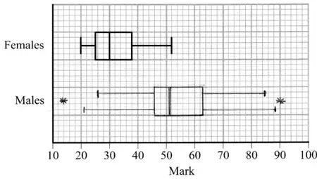
Allow lower whisker to 20.5 and upper whisker to 88.5 Do not allow a mix of whiskers e.g 20.5 and 85 Do not allow both sets of whiskers
M1 A1ft
B1
(5)
Notes
A fully correct box-plot (either version) with no supporting work scores 5/5. Otherwise:
1st M1 for correct attempt to calc’ at least one limit for outliers, ft their quartiles or IQR or award for sight of 20.5 or 88.5
1st A1 for identifying both limits of 20.5 and 88.5
2nd M1 for a box with an upper and a lower whisker(s) with at least 2 correct values (or correct ft) (condone no median marked) (condone 2 upper or 2 lower whiskers)
2nd A1ft for their 20.5 or 26 ,46, 51, 63 and 85 or their 88.5 in appropriate places and readable off their scale. Follow through their 20.5 and their 88.5 only, other values need to be correct. If there are 2 upper or 2 lower whiskers A0
B1 for only 2 outliers appropriately marked at 14 and 90 Do not award if whiskers go beyond these values.
Apply \(\pm\) 0.5 square accuracy for diagram A box plot not on the graph paper can only score the 1st M1A1
Mark scheme (d)
Scheme
Marks
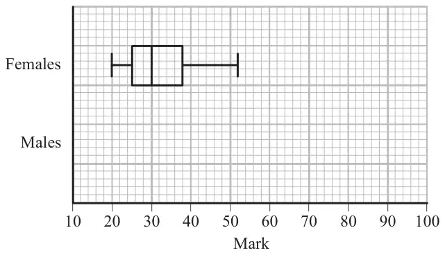
Medians: Median for females lower than males IQR: IQR for females smaller than males. Allow “lower/higher” but not “wider” Range: Range of females is less than males Skewness: Male and female marks are both positively skew Ignore other statements about average, spread, mean, st. Dev, variation, outliers etc
B1ft B1ft
(2)
(11 marks)
Notes
In (d) ft from their diagrams (if no diagram then use their values)
1st B1ft for one correct comment comparing median, IQR , range or skewness
2nd B1ft for a second correct comment comparing median, IQR, range or skewness. Do not allow contradictory statements
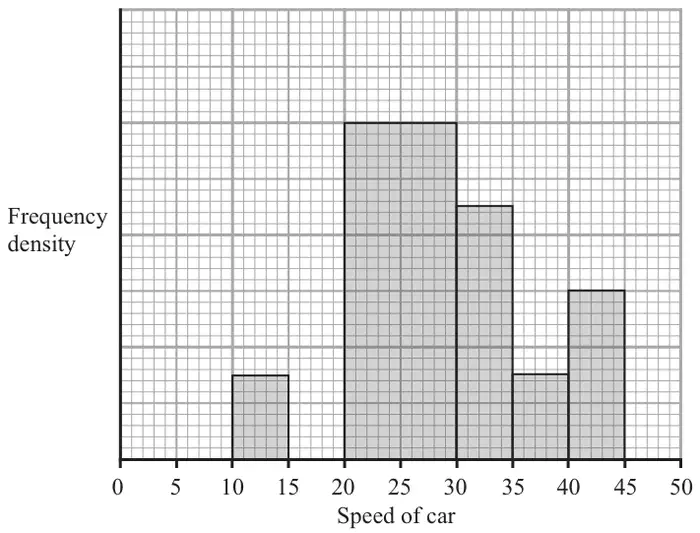
A policeman records the speed of the traffic on a busy road with a 30 mph speed limit. He records the speeds of a sample of 450 cars. The histogram in Figure 2 represents the results.
(a) Calculate the number of cars that were exceeding the speed limit by at least 5 mph in the sample. (4)
(b) Estimate the value of the mean speed of the cars in the sample. (3)
(c) Estimate, to 1 decimal place, the value of the median speed of the cars in the sample. (2)
(d) Comment on the shape of the distribution. Give a reason for your answer. (2)
(e) State, with a reason, whether the estimate of the mean or the median is a better representation of the average speed of the traffic on the road. (2)
Mark scheme (a)
Scheme
Marks
One large square \(= \dfrac{450}{\text{"}22.5\text{"}}\) or one small square \(= \dfrac{450}{\text{"}562.5\text{"}}\) (o.e. e.g. \(\dfrac{\text{"}562.5\text{"}}{450}\))
M1
One large square = 20 cars or one small square = 0.8 cars or 1 car = 1.25 squares
A1
No. > 35 mph is: \(4.5\times\text{"}20\text{"}\) or \(112.5\times\text{"}0.8\text{"}\) (or equivalent e.g. using fd)
dM1
\(=\) 90 (cars)
A1
(4)
Notes
1st M1 for attempt to count squares (accept “22.5” in [22, 23] and “562.5” in [550, 575]) and use 450 to obtain a measure of scale. [If using fd must use 450 to obtain scale factor]
1st A1 for a correct calc. for 20 or 0.8 or 1.25 etc [ May be fd = 4 to 1 large sq. or 0.8 to 1 small sq. May be on the diagram.]
2nd dM1 dep on 1st M1 for correctly counting squares for > 35 mph and forming suitable expr’
2nd A1 for 90 with no incorrect working seen. e.g. \(\dfrac{4.5}{22.5}\times 450\) scores M1A1M1 and A1 when = 90 is seen. Answer only is 4/4
M1 for a full expression for median (using their frequencies). May see e.g. \(25 + \dfrac{75}{120}\times 5\) etc. Do nor accept boundaries of 19.5 or 20.5, these are M0A0
A1 for awrt 28.1 (answer only is 2/2) [For use of \((n + 1)\) accept 28.15 but not 28.2]
1st B1ft for a correct statement about their \(Q_2\) and \(\bar{x}\) [Condone \(Q_2 \approx \bar{x}\) only if \(|Q_2 - \bar{x}| \lt 1\)]. Do not accept an argument based on the shape of the graph alone.
2nd dB1ft dependent on 1st B1 for a compatible description of skewness. F.t. their values
Quartiles If \(Q_1 = 23.4\) and \(Q_3 = 33.7 \sim 33.8\) are seen allow comparison of quartiles for 1st B1 in (d)
Mark scheme (e)
Scheme
Marks
[If chose skew in (d)] median (\(Q_2\)) [If chose symmetric in (d)] mean (\(\bar{x}\))
B1
Since the data is skewed or median not affected by extreme values [Since it uses all the data]
dB1
(2)
(13 marks)
Notes
1st B1 for a correct choice based on their skewness comment in (d). If no choice made in (d) only \(Q_2\)
2. A lake contains 3 species of fish. There are estimated to be 1400 trout, 600 bass and 450 pike in the lake. A survey of the health of the fish in the lake is carried out and a sample of 30 fish is chosen.
(a) Give a reason why stratified random sampling cannot be used. (1)
(b) State an appropriate sampling method for the survey. (1)
(c) Give one advantage and one disadvantage of this sampling method. (2)
(d) Explain how this sampling method could be used to select the sample of 30 fish. You must show your working. (4)
Mark scheme (a)
Scheme
Marks
Sampling frame within each species of fish in the lake impossible to obtain.
B1
(1)
Notes
‘You can’t / it’s very difficult to number all the fish’ or equivalent
Mark scheme (b)
Scheme
Marks
Quota sampling
B1
(1)
Mark scheme (c)
Scheme
Marks
Advantages: Sample can be obtained quickly Costs are kept to a minimum Administration of survey is easy
B1
Disadvantages: Not possible to estimate sampling errors Process not random Surveyor may not be able to identify species of fish easily
B1
(2)
Notes
Correct answer to (b) required. Some detail required.
Mark scheme (d)
Scheme
Marks
Species
Quota
Trout
\(\dfrac{1400}{2450} \times 30 = 17.14\)
Bass
\(\dfrac{600}{2450} \times 30 = 7.35\)
Pike
\(\dfrac{450}{2450} \times 30 = 5.51\)
Fish are caught from the lake until the quota of 17 trout, 7 bass and 6 pike are reached.
B1B1B1
If a fish is caught and the species quota is full, then this is ignored.
B1
(4)
(8 marks)
Notes
1st B1 any one correct calculation seen or implied
2nd B1 all correct to at least 1 dp
3rd B1 for 17,7,6
4th B1 accept equivalent statement. Require comment on what to do with ‘extra fish’.
4. The marks, \(x\), of 45 students randomly selected from those students who sat a mathematics examination are shown in the stem and leaf diagram below.
Mark
Totals
3
6 9 9
(3)
4
0 1 2 2 3 4
(6)
4
5 6 6 6 8
(5)
5
0 2 3 3 4 4
(6)
5
5 5 6 7 7 9
(6)
6
0 0 0 0 1 3 4 4 4
(9)
6
5 5 6 7 8 9
(6)
7
1 2 3 3
(4)
Key (3|6 means 36)
(a) Write down the modal mark of these students. (1)
(b) Find the values of the lower quartile, the median and the upper quartile. (3)
For these students \(\sum x = 2497\) and \(\sum x^2 = 143\,369\)
(c) Find the mean and the standard deviation of the marks of these students. (3)
(d) Describe the skewness of the marks of these students, giving a reason for your answer. (2)
The mean and standard deviation of the marks of all the students who sat the examination were 55 and 10 respectively. The examiners decided that the total mark of each student should be scaled by subtracting 5 marks and then reducing the mark by a further 10%.
(e) Find the mean and standard deviation of the scaled marks of all the students. (4)
Mark scheme (a)
Scheme
Marks
60
B1
(1)
Notes
B1 60 only
Mark scheme (b)
Scheme
Marks
\(Q_1 = 46\)
B1
\(Q_2 = 56\)
B1
\(Q_3 = 64\)
B1
(3)
Notes
Award each B1 for correct answer only in this order.
= 10.342… (\(s\) = 10.459..) anything which rounds to 10.3 (or s = 10.5)
A1
(3)
Notes
M1 for use of correct formula, including square root. Correct answers with no working B1M1A1.
Mark scheme (d)
Scheme
Marks
Mean < median < mode or \(Q_2 - Q_1 \gt Q_3 - Q_2\) with or without their numbers or median closer to upper quartile (than lower quartile) or (mean-median)/sd <0;
B1
negative skew;
B1dep
(2)
Notes
B1 any correct comparison of a pair of mean, median and mode using their values. B1 for ‘negative skew’ or allow (almost) symmetrical dependent upon correct reason.
Mark scheme (e)
Scheme
Marks
mean = \((55 - 5) \times 0.9\)
M1
= 45
A1
sd = \(10 \times 0.9\)
M1
= 9
A1
(4)
(13 marks)
Notes
M1 for (55 or 55.5 - 5)\(\times\)0.9 A1 for the correct answer only. M1 for (10 or 10.3 or 10.5) )\(\times\)0.9 A1 for the correct answer only.
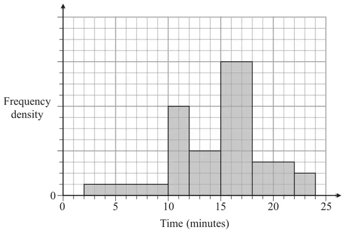
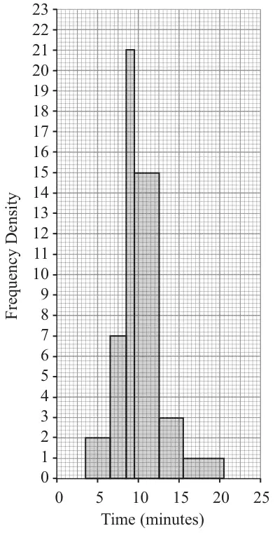
1. The histogram in Figure 1 shows the time, to the nearest minute, that a random sample of 100 motorists were delayed by roadworks on a stretch of motorway.
Figure 1
(a) Complete the table.
Delay (minutes)
Number of motorists
4 – 6
6
7 – 8
9
21
10 – 12
45
13 – 15
9
16 – 20
(2)
(b) Estimate the number of motorists who were delayed between 8.5 and 13.5 minutes by the roadworks. (2)
Mark scheme (a)
Scheme
Marks
14, 5
M1 A1
(2)
Notes
M1 for 2x7 or 14 or 5x1 or 5 A1 for both 14 and 5
Mark scheme (b)
Scheme
Marks
21 + 45 + 3 = 69
M1 A1
(2)
(4 marks)
Notes
M1 for 21+45+(0<frequency <9) A1 for 69 only. 69 no working, award M1A1 Incorrect answer with no working M0A0
5. A class of students had a sudoku competition. The time taken for each student to complete the sudoku was recorded to the nearest minute and the results are summarised in the table below.
Time
Mid-point, \(x\)
Frequency, f
2 - 8
5
2
9 - 12
7
13 - 15
14
5
16 - 18
17
8
19 - 22
20.5
4
23 - 30
26.5
4
(You may use \(\sum \mathrm{f}x^2 = 8603.75\))
(a) Write down the mid-point for the 9 - 12 interval. (1)
(b) Use linear interpolation to estimate the median time taken by the students. (2)
(c) Estimate the mean and standard deviation of the times taken by the students. (5)
The teacher suggested that a normal distribution could be used to model the times taken by the students to complete the sudoku.
(d) Give a reason to support the use of a normal distribution in this case. (1)
On another occasion the teacher calculated the quartiles for the times taken by the students to complete a different sudoku and found
\[Q_1 = 8.5 \qquad Q_2 = 13.0 \qquad Q_3 = 21.0\]
(e) Describe, giving a reason, the skewness of the times on this occasion. (2)
Mark scheme (a)
Scheme
Marks
10.5
B1
(1)
Notes
In parts (a) to (c) a correct answer with no working scores full marks for that value.
M1 for a correct ratio and times 3, ignore the lower boundary for this mark A1 for awrt 15.9 (if \(n\) =30 used) or awrt 16.1 (if \(n\)+1 = 31 is used)
1st M1 for attempt at \(\sum \mathrm{f}x\) (this may be seen in the table as f\(x\): 10, 73.5, 70, 136, 82, 106 [condone 1 slip] or awrt 500) and use of \(\dfrac{\sum \mathrm{f}x}{\sum \mathrm{f}}\) or a correct expression for mean. 1st A1 for awrt 15.9
2nd M1 for an attempt at \(\sigma\) or \(\sigma^2\), can ft their mean, condone mis-labelling \(\sigma^2 = \sqrt{\ldots}\) etc Allow use of their \(\sum \mathrm{f}x^2\) (awrt 9000) 2nd A1ft for a correct expression including square root, ft their mean but not their \(\sum \mathrm{f}x^2\). No label or correct label is OK but wrong label (e.g. \(\sigma^2 = \sqrt{\ldots}\) ) is A0 3rd A1 for awrt 5.78, allow \(s\) = awrt 5.88. SC Allow M1A1A0 for awrt 5.79 if \(\bar{x}\) correct
Mark scheme (d)
Scheme
Marks
Since mean and median are similar (or equal or very close) a normal distribution may be suitable. [Allow mean or median close to mode/modal class]
B1
(1)
Notes
B1 for a reason implying or stating symmetry. "Time is continuous" or “evenly distributed” is B0
Mark scheme (e)
Scheme
Marks
\(Q_3 - Q_2\,(= 8) \gt (4.5 =)\,Q_2 - Q_1\)
M1
Therefore positive skew
A1
(2)
(11 marks)
Notes
M1 for a clear reason or comparison, values not essential but comparison implying they have been found is required. A1 for stating "positive skew". Condone just "positive" but "positive correlation" is A0
Do not allow arguments based on mean and median since this part relates to a different set of data.
5. On a randomly chosen day, each of the 32 students in a class recorded the time, \(t\) minutes to the nearest minute, they spent on their homework. The data for the class is summarised in the following table.
Time, \(t\)
Number of students
10 – 19
2
20 – 29
4
30 – 39
8
40 – 49
11
50 – 69
5
70 – 79
2
(a) Use interpolation to estimate the value of the median. (2)
(b) find the mean and the standard deviation of the times spent by the students on their homework. (3)
(c) Comment on the skewness of the distribution of the times spent by the students on their homework. Give a reason for your answer. (2)
Mark scheme (a)
Scheme
Marks
Median = 32/2 = 16th term (16.5) \(\dfrac{x - 39.5}{49.5 - 39.5} = \dfrac{16 - 14}{25 - 14}\) or \(x = 39.5 + \left(\dfrac{2}{11} \times 10\right)\)
M1
Median = 41.3 ( use of \(n\) + 1 gives 41.8) (awrt 41.3)
A1
(2)
Notes
M1 for an attempt to use interpolation to find the median. Condone use of 39 or 40 for 39.5 e.g. allow \(39 + \dfrac{2}{11} \times 10\) (o.e.) or \(40 + \dfrac{2}{11} \times 10\) (o.e.) to score M1A0 but must have the 10 A1 for awrt 41.3 (or awrt 41.8 if using (\(n\) + 1))
Mark scheme (b)
Scheme
Marks
Mean= \(\dfrac{1414}{32} = 44.1875\) (awrt 44.2)
B1
Standard deviation \(= \sqrt{\dfrac{69378}{32} - \left(\dfrac{1414}{32}\right)^2}\)
M1
= 14.7 (or \(s\) = 14.9)
A1
(3)
Notes
B1 for awrt 44.2 M1 for a correct expression including square root. (Allow ft of their mean) A1 for awrt 14.7 (If using \(s\) for awrt 14.9)
Mid-points: You may see \(\sum t = 1339 \to \bar{t} = 41.8\) and \(\sum t^2 = 62928 \to \sigma\) 14.7 or \(s\) = 14.9 this scores B0 for the mean but can score M1 for a correct st.dev expression and A1 for ans.
Correct answer only in (a) and (b) can score full marks but check (\(n\) +1) case in (a)
Mark scheme (c)
Scheme
Marks
mean > median therefore positive skew
B1ft B1ft
(2)
(7 marks)
Notes
1st B1ft for a correct comparison of their mean and their median (may be in a formula) Calculating median – mean as negative is OK for this B1 but must say +ve skew for 2nd B1 Only allow comparison to be \(\approx 0\) if \(|\text{mean} - \text{median}| \leqslant 0.5\)
2nd B1ft for a correct description of skewness based on their values of mean and median. ft their values for mean and median not their previous calculation/comparison Must be compatible with their previous comparison (if they have one) “Positive skew” with no reason is B0B1 provided you can see their values that imply that. Description should be “positive” or “negative” or “no” skew or “symmetric” “Positive correlation” is B0
Quartiles: 1st B1ft if \(Q_1\) = awrt 32 and \(Q_3\) = awrt 49 seen and a correct comparison made. ft \(Q_2\) 2nd B1ft if \(Q_1\) = awrt 32 or \(Q_3\) = awrt 49 seen and a correct description based on their quartiles and their comparison is made. (Should get “negative skew”)
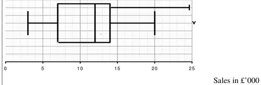
3. Over a long period of time a small company recorded the amount it received in sales per month. The results are summarised below.
Amount received in sales (£1000s)
Two lowest values
3, 4
Lower quartile
7
Median
12
Upper quartile
14
Two highest values
20, 25
An outlier is an observation that falls either 1.5 \(\times\) interquartile range above the upper quartile or 1.5 \(\times\) interquartile range below the lower quartile.
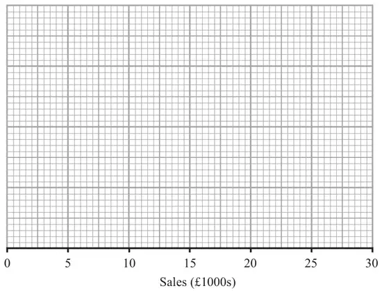
(a) On the graph paper below, draw a box plot to represent these data, indicating clearly any outliers.(5)
(b) State the skewness of the distribution of the amount of sales received. Justify your answer. (2)
(c) The company claims that for 75% of the months, the amount received per month is greater than £10 000. Comment on this claim, giving a reason for your answer. (2)
Mark scheme (a)
Scheme
Marks
Outliers \(14 + 1.5 \times (14 - 7) = 24.5\)
M1
\(7 - 1.5 \times (14 - 7) = -3.5\)
A1
Outlier 25 either upper limit acceptable on diagram
M1 A1ft B1
(5)
Notes
A fully correct box-plot (either version) with no supporting work scores 5/5. Otherwise read on
1st M1 for at least one correct calculation seen 1st A1 for 24.5 and \(-3.5\) (or just negative noted) seen. May be read off the graph. If both values are seen but no calculation is given then M1A1,one value M1A0.
2nd M1 for a box with an upper and a lower whisker(s) with at least 2 correct values (condone no median marked) 2nd A1ft for 3,7, 12, 14 and 20 or 24.5 in appropriate places and readable off their scale If both upper whiskers are seen A0 Apply ft for their whiskers being compatible with their outlier limits e.g. if their lower limit is + 3.5 then a lower whisker ending at 4 or 3.5 is OK
B1 for only one outlier appropriately marked at 25
Apply \(\pm\) 0.5 square accuracy for diagram
Mark scheme (b)
Scheme
Marks
Since \(Q_3 - Q_2 \lt Q_2 - Q_1\). Allow written explanation negatively skew
B1 dB1
(2)
Notes
1st B1 for \(Q_3 - Q_2 \lt Q_2 - Q_1\) statement or an equivalent statement in words Use of \(Q_3 - Q_2 \lt Q_2 - Q_1\) does not require differences to be seen. 2nd dB1 for “negative skew” dependent on suitable reason given above. “correlation” is B0 “positive skew” with a supporting argument based on whiskers can score B1B1 e.g. “right hand whisker is longer than LH one so positive skew” \(Q_3 - Q_2 \lt Q_2 - Q_1\) followed by “positive skew” is B1B0
Mark scheme (c)
Scheme
Marks
not true since the lower quartile is 7000 and therefore 75% above 7000 not 10000 or 10 is inside the box or any other sensible comment
B1 dB1
(2)
(9 marks)
Notes
1st B1 for rejecting the company’s claim 2nd dB1 for an appropriate supporting reason. Dependent on rejecting company’s claim.
2. Keith records the amount of rainfall, in mm, at his school, each day for a week. The results are given below.
2.8 5.6 2.3 9.4 0.0 0.5 1.8
Jenny then records the amount of rainfall, \(x\) mm, at the school each day for the following 21 days. The results for the 21 days are summarised below.
\[\sum x = 84.6\]
(a) Calculate the mean amount of rainfall during the whole 28 days. (2)
Keith realises that he has transposed two of his figures. The number 9.4 should have been 4.9 and the number 0.5 should have been 5.0 Keith corrects these figures.
(b) State, giving your reason, the effect this will have on the mean. (2)
Mark scheme (a)
Scheme
Marks
2.8 + 5.6 + 2.3 + 9.4 + 0.5 + 1.8 + 84.6 = 107
M1
mean = 107 / 28 (= 3.821… ) (awrt 3.8)
A1
(2)
Notes
M1 for a clear attempt to add the two sums. Accept a full expression or 2.8 + 5.6 + …+ 84.6 = \(x\) where \(100 \lt x \lt 110\) i.e. seeing at least two correct terms of Keith’s and the 84.6 with a slip. A1 for awrt 3.8 (Condone 1 dp/2sf here since data is given to 1 dp or 2 sf) Accept \(\dfrac{107}{28}\) or \(3\dfrac{23}{28}\) or any exact equivalent
Correct answer implies M1A1
Mark scheme (b)
Scheme
Marks
It will have no effect since one is 4.5 under what it should be and the other is 4.5 above what it should be.
B1 dB1
(2)
(4 marks)
Notes
1st B1 for clearly stating that it will have no effect. (“roughly the same” is B0 B0) 2nd dB1 for a supporting reason that mentions the fact that the increase and decrease are the same and gives some numerical value(s) to support this. e.g. Sum of Keith’s observations is still 22.4 ( or mean is still 3.2) or Sum is still 107 or \(9.4 - 4.9 = 5 - 0.5\) (o.e.) This second B1 is dependent on their saying there is no effect so B0B1 is not possible.
1st M1 for reasonable attempt at \(\sum x\) and /56 2nd M1 for a method for \(\sigma\) or \(s\), \(\sqrt{\phantom{x}}\) is required Typical errors \(\sum (\mathrm{f}x)^2 = 354806.3\) M0, \(\sum \mathrm{f}^2x = 13922.5\) M0 and \((\sum \mathrm{f}x)^2 = 1733172\) M0 Correct answers only, award full marks.
Use of \(\sum \mathrm{f}(x - \bar{x})^2\) = awrt 6428.75 for B1 (this note is printed under (d) in the mark scheme)
lcb can be 20, 20.5 or 21, width can be 4 or 5 and the fraction part of the formula correct for M1 - Allow 28.5 in fraction that gives awrt 23.9 for M1A1
M1 for attempting a test for skewness using quartiles or mean and median. Provided median greater than 22.55 and less than 29.3 award for M1 for \(Q_3 - Q_2 \lt Q_2 - Q_1\) without values as a valid reason. SC Accept mean close to median and no skew oe for M1A1
3. The birth weights, in kg, of 1500 babies are summarised in the table below.
Weight (kg)
Midpoint, \(x\) kg
Frequency, f
0.0 – 1.0
0.50
1
1.0 – 2.0
1.50
6
2.0 – 2.5
2.25
60
2.5 – 3.0
280
3.0 – 3.5
3.25
820
3.5 – 4.0
3.75
320
4.0 – 5.0
4.50
10
5.0 – 6.0
3
[You may use \(\sum \mathrm{f}x = 4841\) and \(\sum \mathrm{f}x^2 = 15\,889.5\)]
(a) Write down the missing midpoints in the table above. (2)
(b) Calculate an estimate of the mean birth weight. (2)
(c) Calculate an estimate of the standard deviation of the birth weight. (3)
(d) Use interpolation to estimate the median birth weight. (2)
(e) Describe the skewness of the distribution. Give a reason for your answer. (2)
Mark scheme (a)
Scheme
Marks
2.75 or \(2\tfrac{3}{4}\), 5.5 or 5.50 or \(5\tfrac{1}{2}\)
B1 B1
(2)
Mark scheme (b)
Scheme
Marks
Mean birth weight \(= \dfrac{4841}{1500} = 3.227\dot{3}\) awrt 3.23
M1 A1
(2)
Notes
M1 for a correct expression for mean. Answer only scores both.
Mark scheme (c)
Scheme
Marks
Standard deviation \(= \sqrt{\dfrac{15889.5}{1500} - \left(\dfrac{4841}{1500}\right)^2} = 0.421093\ldots\) or \(s = 0.4212337\ldots\)
M1 A1ft A1
(3)
Notes
M1 for a correct expression (ft their mean) for sd or variance. Condone mis-labelling eg sd=… with no square root or no labelling
1st A1ft for a correct expression (ft their mean) including square root and no mis-labelling Allow 1st A1 for \(\sigma^2 = 0.177\ldots \to \sigma = 0.42\ldots\)
M1 for a correct expression (allow 403.5 i.e. use of \(n + 1\)) but must have 3.00, 820 and 0.5
A1 for awrt 3.25 provided M1 is scored. NB 3.25 with no working scores 0/2 as some candidates think mode is 3.25.
Mark scheme (e)
Scheme
Marks
Mean(3.23)<Median(3.25) (or very close)
B1ft
Negative Skew (or symmetrical)
dB1ft
(2)
(11 marks)
Notes
1st B1ft for a comparison of their mean and median (may be in a formula but if ±(mean - median) is calculated that’s OK. We are not checking the value but the sign must be consistent.) Also allow for use of quartiles provided correct values seen: \(Q_1 = 3.02, Q_3 = 3.47\) [They should get \((0.22 =)\, Q_3 - Q_2 \lt Q_2 - Q_1\, (= 0.23)\) and say (slight) negative skew or symmetric]
2nd dB1ft for a compatible comment based on their comparison. Dependent upon a suitable, correct comparison. Mention of “correlation” rather than “skewness” loses this mark.
2. The 19 employees of a company take an aptitude test. The scores out of 40 are illustrated in the stem and leaf diagram below.
2|6 means a score of 26
0
7
(1)
1
88
(2)
2
4468
(4)
3
2333459
(7)
4
00000
(5)
Find
(a) the median score, (1)
(b) the interquartile range. (3)
The company director decides that any employees whose scores are so low that they are outliers will undergo retraining.
An outlier is an observation whose value is less than the lower quartile minus 1.0 times the interquartile range.
(c) Explain why there is only one employee who will undergo retraining. (2)
(d) On the graph paper, draw a box plot to illustrate the employees’ scores. (3)
Mark scheme (a)
Scheme
Marks
Median is 33
B1
(1)
Mark scheme (b)
Scheme
Marks
\(Q_1 = 24,\ Q_3 = 40,\ \text{IQR} = 16\)
B1 B1 B1ft
(3)
Notes
1st B1 for \(Q_1 = 24\) and 2nd B1 for \(Q_3 = 40\)
3rd B1ft for their IQR based on their lower and upper quartile. Calculation of range (40 – 7 = 33) is B0B0B0
Answer only of IQR = 16 scores 3/3. For any other answer we must see working in (b) or on stem and leaf diagram
Mark scheme (c)
Scheme
Marks
\(Q_1 - \text{IQR} = 24 - 16 = 8\)
M1
So 7 is only outlier
A1ft
(2)
Notes
M1 for evidence that \(Q_1\)-IQR has been attempted, their “8” (>7) seen or clearly attempted is sufficient
A1ft must have seen their “8” and a suitable comment that only one person scored below this.
Mark scheme (d)
Scheme
Marks
(accept either whisker)
B1ft (Box) B1 (Outlier) B1ft (Whisker)
(3)
(9 marks)
Notes
1st B1ft for a clear box shape and ft their \(Q_1, Q_2\) and \(Q_3\) readable off the scale. Allow this mark for a box shape even if \(Q_3 = 40\), \(Q_1 = 7\) and \(Q_2 = 33\) are used
2nd B1 for only one outlier appropriately marked at 7
3rd B1ft for either lower whisker. If they choose the whisker to their lower limit for outliers then follow through their “8”. (There should be no upper whisker unless their \(Q_3 \lt 40\), in which case there should be a whisker to 40)
A typical error in (d) is to draw the lower whisker to 7, this can only score B1B0B0
1. A telephone directory contains 50 000 names. A researcher wishes to select a systematic sample of 100 names from the directory.
(a) Explain in detail how the researcher should obtain such a sample. (2)
(b) Give one advantage and one disadvantage of
(i) quota sampling,
(ii) systematic sampling. (4)
Mark scheme (a)
Scheme
Marks
Randomly select a number between 00 and 499 (001 and 500)
B1
select every 500th person
B1
(2)
Notes
1st B1 for idea of using random numbers to select the first from 1 - 500 (o.e.)
2nd B1 for selecting every 500th (name on the list)
If they are clearly trying to carry out stratified sample then score B0B0
Mark scheme (b)
Scheme
Marks
(i) Quota Advantage: Representative sample can be achieved (with small sample size) Cheap (costs kept to a minimum) not “quick” Administration relatively easy
B1
Disadvantage Not possible to estimate sampling errors (due to lack of randomness) Not a random process Judgment of interviewer can affect choice of sample – bias Non-response not recorded Difficulties of defining controls e.g. social class
B1
(2)
(ii) Systematic Advantage: Simple or easy to use not “quick” or “cheap” or “efficient” It is suitable for large samples (not populations)
B1
Disadvantage Only random if the ordered list is (truly) random Requires a list of the population or must assign a number to each member of the pop.
B1
(2)
(6 marks)
Notes
Score B1 for any one line
(i) 1st B1 for Quota advantage 2nd B1 for Quota disadvantage
(ii) 3rd B1 for Systematic Advantage 4th B1 for Systematic Disadvantage
5. A researcher is hired by a cleaning company to survey the opinions of employees on a proposed pension scheme. The company employs 55 managers and 495 cleaners.
To collect data the researcher decides to give a questionnaire to the first 50 cleaners to leave at the end of the day.
(a) Give 2 reasons why this method is likely to produce biased results. (2)
(b) Explain briefly how the researcher could select a sample of 50 employees using
(i) a systematic sample,
(ii) a stratified sample. (6)
Using the random number tables in the formulae book, and starting with the top left hand corner (8) and working across, 50 random numbers between 1 and 550 inclusive were selected. The first two suitable numbers are 384 and 100.
(c) Find the next two suitable numbers. (2)
Mark scheme (a)
Scheme
Marks
Only cleaners - no managers i.e. not all types. OR Not a random sample
B1g
1st 50 may be in same shift/group/share same views. OR Not a random sample (Allow “not a representative sample” in place of “not a random sample”)
B1h
(2)
Notes
After 1st B1, comments should be in context, i.e. mention cleaners, managers, types of worker etc
1st B1g for one row 2nd B1h for both rows. “Not a random sample” only counts once. Score B1B0 or B1B1 or B0B0 on EPEN
Mark scheme (b)
Scheme
Marks
(i) Label employees (1-550) or obtain an ordered list
B1
Select first using random numbers (from 1 - 11)
B1
Then select every 11th person from the list
B1
(ii) Label managers (1-55) and cleaners (1-495)
M1
Use random numbers to select…
M1
…5 managers and 45 cleaners
A1
(6)
Notes
(i) 1st B1 for idea of labelling or getting an ordered list. No need to see 1-550. 2nd B1 selecting first member of sample using random numbers (1-11 need not be mentioned) 3rd B1 selecting every \(n\)th where \(n = 11\).
(ii) 1st M1 for idea of two groups and labelling both groups. (Actual numbers used not required) 2nd M1 for use of random numbers within each strata. Don’t give for SRS from all 550. “Assign random numbers to managers and cleaners” scores M0M1 A1 for 5 managers and 45 cleaners. (This mark is dependent upon scoring at least one M)
Each cooker produced at GT Engineering is stamped with a unique serial number. GT Engineering produces cookers in batches of 2000. Before selling them, they test a random sample of 5 to see what electric current overload they will take before breaking down.
(b) Give one reason, other than to save time and cost, why a sample is taken rather than a census. (1)
(c) Suggest a suitable sampling frame from which to obtain this sample. (1)
(d) Identify the sampling units. (1)
Mark scheme (a)
Scheme
Marks
A census is when every member of the population is investigated.
B1
(1)
Notes
B1 Need one word from each group (1) Every member /all items / entire /oe (2) population/collection of individuals/sampling frame/oe
enumerating the population on its own gets B0
Mark scheme (b)
Scheme
Marks
There would be no cookers left to sell.
B1
(1)
Notes
B1 Idea of Tests to destruction. Do not accept cheap or quick
Mark scheme (c)
Scheme
Marks
A list of the unique identification numbers of the cookers.
B1
(1)
Notes
B1 Idea of list/ register/database of cookers/serial numbers
Mark scheme (d)
Scheme
Marks
A cooker
B1
(1)
(4 marks)
Notes
B1 cooker(s) / serial number(s)
The sample of 5 cookers or every 400th cooker gets B1
(a) Give two reasons to justify the use of statistical models. (2)
It has been suggested that there are 7 stages involved in creating a statistical model. They are summarised below, with stages 3, 4 and 7 missing.
Stage 1. The recognition of a real-world problem. Stage 2. A statistical model is devised. Stage 3. Stage 4. Stage 5. Comparisons are made against the devised model. Stage 6. Statistical concepts are used to test how well the model describes the real-world problem. Stage 7.
(b) Write down the missing stages. (3)
Mark scheme (a)
Scheme
Marks
Used to simplify or represent a real world problem Cheaper or quicker or easier (than the real situation) or more easily modified To improve understanding of the real world problem Used to predict outcomes from a real world problem (idea of predictions)
B1 B1
(2)
Notes
B1B1 (any two lines)
1stB1 For one line 2ndB1 For a second line Be generous for 1st B1 but stricter for B1B1
Mark scheme (b)
Scheme
Marks
(3 or 4) Model used to make predictions. (Idea of predicted values based on the model)
B1
(4 or 3) (Experimental) data collected
B1
(7) Model is refined.
B1
(3)
(5 marks)
Notes
1st & 2ndB1 These two points can be interchanged. Idea of values from (experimental) data and predicted values based on the model.
1stB1 for predicted values from model e.g. “model used to gain suitable data”
2ndB1 for data collected. Idea of experimental data but “experiment” needn’t be explicitly seen
3rdB1 This should be stage 7. Idea of refinement or revision or adjustment
5. A teacher recorded, to the nearest hour, the time spent watching television during a particular week by each child in a random sample. The times were summarised in a grouped frequency table and represented by a histogram.
One of the classes in the grouped frequency distribution was 20–29 and its associated frequency was 9. On the histogram the height of the rectangle representing that class was 3.6 cm and the width was 2 cm.
(a) Give a reason to support the use of a histogram to represent these data. (1)
(b) Write down the underlying feature associated with each of the bars in a histogram. (1)
(c) Show that on this histogram each child was represented by 0.8 cm2. (3)
The total area under the histogram was 24 cm2.
(d) Find the total number of children in the group. (2)
Mark scheme (a)
Scheme
Marks
Time is a continuous variable or data is in a grouped frequency table
B1
(1)
Mark scheme (b)
Scheme
Marks
Area is proportional to frequency or \(A \propto f\) or \(A = kf\)
B1
(1)
Notes
1stB1 for one of these correct statements. “Area proportional to frequency density” or “Area = frequency” is B0
Mark scheme (c)
Scheme
Marks
\(3.6 \times 2 = 0.8 \times 9\)
M1 dM1
1 child represented by 0.8
A1 cso
(3)
Notes
1stM1 for a correct combination of any 2 of the 4 numbers: 3.6, 2, 0.8 and 9 e.g. \(3.6 \times 2\) or \(\dfrac{3.6}{0.8}\) or \(\dfrac{0.8}{2}\) etc BUT e.g. \(\dfrac{3.6}{2}\) is M0
2ndM1 dependent on 1st M1 and for a correct combination of 3 numbers leading to 4th. May be in separate stages but must see all 4 numbers
A1cso for fully correct solution. Both Ms scored, no false working seen and comment required.
A1 awrt 26.7 (N.B. Use of 60.5 gives 26.825… so allow awrt 26.8)
M1 for (19.5 or 20) \(+ \dfrac{(60 - 29)}{43} \times 10\) or better. Allow 60.5 giving awrt 26.8 for M1A1 Allow their \(0.5n\) [or \(0.5(n + 1)\)] instead of 60 [or 60.5] for M1.
Mark scheme (c)
Scheme
Marks
\(\mu = \dfrac{3550}{120} = 29.5833\ldots\) or \(29\tfrac{7}{12}\)
\(\sigma = 16.5829\ldots\) or \((s = 16.652\ldots)\)
A1
(3)
Notes
B1 awrt 29.6
A1 awrt 16.6 (or \(s\) = 16.7)
M1 for a correct expression for \(\sigma, \sigma^2, s\) or \(s^2\). NB \(\sigma^2 = 274.99\) and \(s^2 = 277.30\) Condone poor notation if answer is awrt16.6 (or 16.7 for \(s\))
Mark scheme (d)
Scheme
Marks
\(\dfrac{3(29.6 - 26.7)}{16.6}\)
M1A1ft
\(= 0.52\ldots\)
A1
(3)
Notes
A1 awrt 0.520 (or with \(s\) awrt 0.518) (N.B. 60.5 in (b) …awrt 0.499 [or with \(s\) awrt 0.497])
M1 for attempt to use this formula using their values to any accuracy. Condone missing 3. 1stA1ft for using their values to at least 3sf. Must have the 3. 2ndA1 for using accurate enough values to get awrt 0.520 (or 0.518 if using \(s\)) NB Using only 3 sf gives 0.524 and scores M1A1A0
Mark scheme (e)
Scheme
Marks
0.520 > 0
B1ft
So it is consistent with (a)
dB1ft
(2)
Notes
B1ft correct statement about their (d) being >0 or < 0
dB1ft ft their (d)
1stB1 for saying or implying correct sign for their (d). B1g and B1ft. Ignore “correlation” if seen. 2ndB1 for a comment about consistency with their (d) and (a) being positive skew, ft their (d) only This is dependent on 1st B1: so if (d)>0, they say yes, if (d)<0 they say no.
Mark scheme (f)
Scheme
Marks
Use Median
B1
Since the data is skewed or less affected by outliers/extreme values
dB1
(2)
Notes
2ndB1 is dependent upon choosing median.
Mark scheme (g)
Scheme
Marks
If the data are symmetrical or skewness is zero or normal/uniform distribution (“mean =median” or “no outliers” or “evenly distributed” all score B0)
2. Sunita and Shelley talk to one another once a week on the telephone. Over many weeks they recorded, to the nearest minute, the number of minutes spent in conversation on each occasion. The following table summarises their results.
Time (to the nearest minute)
Number of Conversations
5–9
2
10–14
9
15–19
20
20–24
13
25–29
8
30–34
3
Two of the conversations were chosen at random.
(a) Find the probability that both of them were longer than 24.5 minutes. (2)
The mid-point of each class was represented by \(x\) and its corresponding frequency by \(f\), giving \(\Sigma fx = 1060\).
(b) Calculate an estimate of the mean time spent on their conversations. (2)
During the following 25 weeks they monitored their weekly conversations and found that at the end of the 80 weeks their overall mean length of conversation was 21 minutes.
(c) Find the mean time spent in conversation during these 25 weeks. (4)
(d) Comment on these two mean values. (2)
Mark scheme (a)
Scheme
Marks
\(\mathrm{P}(\text{both longer than } 24.5) = \dfrac{11}{55} \times \dfrac{10}{54} = \dfrac{1}{27}\) or \(0.\dot{0}3\dot{7}\) or 0.037
M1A1
(2)
Notes
M1 2 fracs × w/o rep.
A1 awrt 0.037
Mark scheme (b)
Scheme
Marks
Estimate of mean time spent on their conversations is \(\bar{x} = \dfrac{1060}{55} = 19\tfrac{3}{11}\) or \(19.\dot{2}\dot{7}\) or 19.3
M1A1
(2)
Notes
M1A1 1060/total, awrt 19.3 or 19mins 16s
Mark scheme (c)
Scheme
Marks
\(\dfrac{1060 + \sum fy}{80} = 21\)
B1
\(\sum fy = 620\)
M1
\(\therefore \bar{y} = \dfrac{620}{25} = 24.8\)
M1A1
(4)
Notes
B1 \(21 \times 80 = 1680\)
M1 Subtracting ‘their 1060’
M1A1 Dividing their 620 by 25
Mark scheme (d)
Scheme
Marks
Increase in mean value.
B1
Length of conversations increased considerably during 25 weeks relative to 55 weeks
Advantages: – does not require the existence of a population list (sampling frame) – field work can be done quickly as representative sample can be achieved with a small sample size – costs kept to a minimum (cheaply) – administration relatively easy – non-response not an issue any one
B1
Disadvantages: – not possible to estimate sampling errors – interviewer choice and may not be able to judge easily / may lead to bias – non-response not recorded – non-random process any one
B1
(2)
Mark scheme (b)
Scheme
Marks
Advantages: – random process so possible to estimate sampling errors – free from bias any one
B1
Disadvantages: – not suitable when sample size is large – sampling frame required which may not exist or may be difficult to construct for a large population. any one
(a) Describe the main features and uses of a box plot. (3)
Children from schools \(A\) and \(B\) took part in a fun run for charity. The times, to the nearest minute, taken by the children from school \(A\) are summarised in Figure 1.
Figure 1
(b)
(i) Write down the time by which 75% of the children in school \(A\) had completed the run.
(ii) State the name given to this value. (2)
(c) Explain what you understand by the two crosses (×) on Figure 1. (2)
For school \(B\) the least time taken by any of the children was 25 minutes and the longest time was 55 minutes. The three quartiles were 30, 37 and 50 respectively.
(d) Draw a box plot to represent the data from school \(B\). (4)
(e) Compare and contrast these two box plots. (4)
Mark scheme (a)
Scheme
Marks
Indicates max / median / min / upper quartile/ lower quartile (2 or more) Indicates outliers (or equivalent description) Illustrates skewness (or equivalent description e.g. shape) Allows comparisons Indicates range / IQR / spread
B1 B1 B1
(3)
Notes
B1B1B1 Any 3 rows
Mark scheme (b)
Scheme
Marks
(i) 37 (minutes)
B1
(ii) Upper quartile or \(\mathrm{Q}_3\) or third quartile or 75th percentile or \(\mathrm{P}_{75}\)
B1
(2)
Mark scheme (c)
Scheme
Marks
Outliers How to calculate correctly ‘Observations that are very different from the other observations and need to be treated with caution’ These two children probably walked / took a lot longer
B1 B1
(2)
Notes
B1B1 Any 2
Mark scheme (d)
Scheme
Marks
Box & median & whiskers
M1
Sensible scale
B1
30, 37, 50
B1
25, 55
B1
(4)
Mark scheme (e)
Scheme
Marks
Children from school A generally took less time 50% of B \(\leqslant\) 37 mins, 75% of A < 37 mins (similarly for 30) Median/Q1/Q3 of A < median/Q1/Q3 of B (1 or more) A has outliers, (B does not) Both positive skew IQR of A<IQR of B, range of A>range of B
1. A school has 15 classes and a sixth form. In each class there are 30 students. In the sixth form there are 150 students. There are equal numbers of boys and girls in each class. There are equal numbers of boys and girls in the sixth form. The head teacher wishes to obtain the opinions of the students about school uniforms.
Explain how the head teacher would take a stratified sample of size 40. (7)
Mark scheme
Scheme
Marks
Total in School = \((15 \times 30) + 150 = 600\)
B1
random sample of \(\dfrac{30}{600} \times 40\) (Use of \(\dfrac{40}{\text{their } 600}\)) \(= \underline{2}\) from each of the 15 classes
M1 A1
random sample of \(\dfrac{150}{600} \times 40\) Either \(= \underline{10}\) from sixth form;
A1
Label the boys in each class from 1 – 15 and the girls from 1 – 15. use random numbers to select 1 girl and 1 boy
B1 B1
Label the boys in the sixth form from 1 – 75 and the girls from 1 – 75. use random numbers to select 5 different boys and 5 different girls.
1. Over a period of time, the number of people \(x\) leaving a hotel each morning was recorded. These data are summarised in the stem and leaf diagram below.
Number leaving
\(3 \mid 2\) means 32
Totals
2
7 9 9
(3)
3
2 2 3 5 6
(5)
4
0 1 4 8 9
(5)
5
2 3 3 6 6 6 8
(7)
6
0 1 4 5
(4)
7
2 3
(2)
8
1
(1)
For these data,
(a) write down the mode, (1)
(b) find the values of the three quartiles. (3)
Given that \(\Sigma x = 1335\) and \(\Sigma x^2 = 71\,801\), find
(c) the mean and the standard deviation of these data. (4)
4. Aeroplanes fly from City \(A\) to City \(B\). Over a long period of time the number of minutes delay in take-off from City \(A\) was recorded. The minimum delay was 5 minutes and the maximum delay was 63 minutes. A quarter of all delays were at most 12 minutes, half were at most 17 minutes and 75% were at most 28 minutes. Only one of the delays was longer than 45 minutes.
An outlier is an observation that falls either \(1.5 \times\) (interquartile range) above the upper quartile or \(1.5 \times\) (interquartile range) below the lower quartile.
(a) On the graph paper opposite draw a box plot to represent these data. (7)
(b) Comment on the distribution of delays. Justify your answer. (2)
(c) Suggest how the distribution might be interpreted by a passenger who frequently flies from City \(A\) to City \(B\). (1)
Mark scheme (a)
Scheme
Marks
\(1.5(Q_3 - Q_1) = 1.5(28 - 12) = 24\)
B1
\(Q_3 + 24 = 52 \Rightarrow 63\) is an outlier
M1, A1
\(Q_1 - 24 \lt 0 \Rightarrow\) no outliers
A1
Box plot
M1 A1 A1
(7)
Notes
B1 may be implied
M1, A1 att \(Q_3 + \ldots\) or \(Q_1 - \ldots\), 52 and −12 or <0 or evidence of no lower outliers
A1 63 is an outlier
The diagram for the box plot marks (M1 A1 A1) is blank in the printed mark scheme.
Mark scheme (b)
Scheme
Marks
Distribution is +ve skew; \(Q_2 - Q_1\ (5) \lt Q_3 - Q_2\ (11)\);
B1; B1
(2)
Mark scheme (c)
Scheme
Marks
Many delays are small so passengers should find these acceptable or sensible comment in the context of the question.
2. The number of caravans on Seaview caravan site on each night in August last year is summarised in the following stem and leaf diagram.
Caravans
\(1 \mid 0\) means 10
Totals
1
0 5
(2)
2
1 2 4 8
(4)
3
0 3 3 3 4 7 8 8
(8)
4
1 1 3 5 8 8 8 9 9
(9)
5
2 3 6 6 7
(5)
6
2 3 4
(3)
(a) Find the three quartiles of these data. (3)
During the same month, the least number of caravans on Northcliffe caravan site was 31. The maximum number of caravans on this site on any night that month was 72. The three quartiles for this site were 38, 45 and 52 respectively.
(b) On graph paper and using the same scale, draw box plots to represent the data for both caravan sites. You may assume that there are no outliers. (6)
(c) Compare and contrast these two box plots. (3)
(d) Give an interpretation to the upper quartiles of these two distributions. (2)
The marks for (b) are handwritten on the scheme’s diagram.
(corrected from the printed mark scheme: the handwritten list reads “31, 79” for the Northcliffe end points; the question gives the maximum as 72, as marked on the diagram)
Mark scheme (c)
Scheme
Marks
Median of Northcliffe is greater than median of Seaview. Upper quartiles are the same IQR of Northcliffe is less than IQR of Seaview Northcliffe positive skew, Seaview negative skew
19 The table represents the frequency distribution of the CO2 emissions, \(x\) g/km of all of the electric and electric/petrol BMW cars in the Large Data Set that were registered in the South-West in 2016.
\(x\)
0
13
45
49
77
78
Frequency
1
2
3
9
2
2
(a) State the number of electric cars in the distribution. [1 mark]
(b) Find the mean of the CO2 emissions. [1 mark]
(c) Find the standard deviation of the CO2 emissions. [1 mark]
(d) Explain why it is not valid to compare the results from part (b) and part (c) with the mean and standard deviation of the CO2 emissions of the electric and electric/petrol BMW cars in the Large Data Set that were registered in the South-West in 2002. [1 mark]
Mark scheme (a)
Scheme
Marks
AO
Deduces 1
B1
2.2a
(1)
Typical solution
1
Mark scheme (b)
Scheme
Marks
AO
Obtains 48 CAO
B1
1.1b
(1)
Typical solution
Mean = 48
Mark scheme (c)
Scheme
Marks
AO
Obtains AWRT 20.9 Accept AWRT 21.4
B1
1.1b
(1)
Typical solution
Standard deviation = 20.9
Mark scheme (d)
Scheme
Marks
AO
Explains why it is not valid to make the comparison. Must be clear that neither propulsion type OE is in the 2002 data.
E1
2.4
(1)
(4 marks)
Typical solution
The 2002 data does not contain any electric or electric/petrol cars.
17 The owner of a shop recorded the average daily wind speed in mph and the total sales of raincoats in pounds over a period of 6 months.
The data from a random selection of 15 days from the 6-month period is shown in the scatter diagram.
One of the points on the scatter diagram is an outlier.
(a) State the letter from the diagram which corresponds to this outlier. [1 mark]
(b) State the effect on the numerical value of the correlation coefficient if the outlier was removed from the data. [1 mark]
(c) Describe, in context, the correlation indicated by the scatter diagram. [1 mark]
(d) The owner of the shop claims that the scatter diagram proves that windier days cause lower sales of raincoats.
Comment on the validity of this claim. [1 mark]
Mark scheme (a)
Scheme
Marks
AO
States A
B1
2.2a
(1)
Typical solution
A
Mark scheme (b)
Scheme
Marks
AO
Explains that the value would become more negative or strong negative OE Accept smaller/decrease
E1
2.4
(1)
Typical solution
The value would become more negative
Mark scheme (c)
Scheme
Marks
AO
Describes the correlation in context. Require ‘sale(s)’ and ‘wind speed’ Do not accept ‘number’ /’amount’ Accept negative correlation (with ‘sale(s)’ and ‘wind speed’)
Do not accept ‘number’/’amount’
E1
2.2b
(1)
Typical solution
The higher the wind speed the lower the daily sales of raincoats
Mark scheme (d)
Scheme
Marks
AO
States claim is not valid OE, with a comment; E.g.
Accept it may be valid but the scatter diagram does not prove it.
E1
2.2b
(1)
(4 marks)
Typical solution
This claim is not valid. The scatter diagram cannot prove causality, there could be another factor which is causing the fall in sales, e.g. amount of rainfall
16 An investigation into the hydrocarbon emissions, \(X\) g/km, from cars in the Large Data Set was carried out.
The results are summarised below.
\[\sum x = 128.657 \qquad \sum x^2 = 8.701\,707 \qquad n = 2405\]
where \(n\) is the total number of cars which had a measured hydrocarbon emission in the Large Data Set.
(a)
(i) Find the mean of \(X\) [1 mark]
(ii) Find the standard deviation of \(X\) [2 marks]
(b)
(i) The Large Data Set is a sample taken from the entire UK Department for Transport Stock Vehicle Database.
It is claimed that the values in part (a)(i) and part (a)(ii) obtained from the Large Data Set should be reliable estimates for the mean and standard deviation of the hydrocarbon emissions for the entire UK Department for Transport Stock Vehicle Database.
State, with a reason, whether this claim is likely to be correct. [1 mark]
(ii) State one type of emission where more than 80% of the data is known for cars in the entire UK Department for Transport Stock Vehicle Database. [1 mark]
Mark scheme (a)
Scheme
Marks
AO
(i) Obtains correct mean AWFW [0.053, 0.054]
B1
1.1b
(1)
(ii) Obtains a value of the standard deviation in the range [0.0265, 0.0285]
B1
1.1b
Obtains value of the standard deviation AWRT 0.0275
(i) States that the claim is/may be incorrect. With a valid reason Eg Not every make of car is included in the LDS LDS does not reflect number of electric, gas/petrol in UK database Not every region is included in the LDS LDS only comes from 2 years LDS is a small sample compared to the entire UK database
E1
2.2b
(1)
(ii) States CO2, CO or NOX
B1
1.2
(1)
(5 marks)
Typical solution
(i)
The LDS does not include cars from every region of the UK, so the claim may be incorrect.
Gives any correct advantage of a stratified sample Accept: Provides greater precision/reliability The sample is representative of the population/each (year) group Unbiased
19 A comparison of the masses (in kg) of convertible cars was made using the Large Data Set.
A sample of 20 masses was chosen from both the 2002 data and the 2016 data.
The masses of the 20 cars in each sample were used to create a box plot for each year.
The box plots were labelled Box Plot A and Box Plot B as shown in the diagram below.
(a) Estimate the median of the masses from Box Plot A [1 mark]
(b) It is claimed that Box Plot B must be incorrectly drawn.
(i) Give a reason why this claim was made. [1 mark]
(ii) Comment on the validity of this claim. [1 mark]
(c) It is claimed that Box Plot B must be from the 2002 data. Give a reason why this claim is correct. [1 mark]
Mark scheme (a)
Scheme
Marks
AO
Estimates median correctly AWFW 1650 to 1675 Condone missing units
B1
1.1b
(1)
Typical solution
Median = 1662.5kg
Mark scheme (b)
Scheme
Marks
AO
(i) Correctly identifies zero mass implied from the Box Plot
Accept masses should be at least 75kg (due to inclusion of mass of driver of 75kg in data)
B1
2.2a
(1)
(ii) Argues that the claim is incorrect with the correct reason
E1
2.4
(1)
Typical solution
(i)
The Box Plot implies that there is at least one car of zero mass which is not possible
(ii)
There are car masses of zero in the Large Data Set
So, the claim is incorrect
Mark scheme (c)
Scheme
Marks
AO
Explains that the 2002 data is the only one of the two data sets to contain zero masses Or Gives a valid reason for Box Plot B being from the 2002 data or for Box Plot A being from 2016. The reason must be justified from the relevant Box Plot
E1
2.4
(1)
(4 marks)
Typical solution
The 2002 data is the only one of the two data sets to contain zeros in the masses of cars field
14 The manager of a factory wants to introduce a bonus scheme.
The factory has 65 employees who work in production and 28 employees who work in the office.
The manager decides to collect the opinions of a sample of these 93 employees.
(a) Explain how the manager could collect a simple random sample of 20 employees. [3 marks]
(b) The manager collected a simple random sample of 20 employees.
The manager noticed that all 20 of the employees in the sample worked in production and therefore the sample was not representative.
State a different method of sampling that would give a representative sample. [1 mark]
Mark scheme (a)
Scheme
Marks
AO
Sets up the numbering of the population (allow 00 to 92) Allow 01 to 93
E1
2.4
Explains how the calculator (random number generator) will be used to generate random numbers (two-digit PI by between 1 and 93 or in this range or ignore numbers out of range or using these numbers) If using random number tables must state 2-digit numbers OE
E1
2.4
Explains how to deal with repeats (PI) and identify 20 different employees/numbers
E1
2.4
(3)
Typical solution
Number the employees from 1 to 93
Choose random numbers from the calculator in this range
Ignore repeats and continue until 20 different employees have been selected
13 Two random samples of 12 NOX emissions (in g/km) were taken from the Large Data Set.
One sample was taken from the 2002 data and the other sample from the 2016 data.
The sample data are shown below:
2002
0.031
0.019
0.091
0.025
0.030
0.061
0.047
0.029
0.059
0.363
0.330
0.376
2016
0.005
0.047
0.053
0.063
0.026
0.013
0.058
0.012
0.010
0.010
0.008
0.008
The mean and standard deviation of the 2002 sample data are 0.122 and 0.137 respectively.
(a) Find the mean and standard deviation of the 2016 sample data giving your answers correct to three decimal places. [2 marks]
(b) Siti claims these samples show that, on average, the NOX emissions across all makes of car in all areas of the UK have fallen by over 75% between 2002 and 2016.
(i) Show how Siti’s claim of ‘over 75%’ has been obtained. [2 marks]
(ii) Using your knowledge of the Large Data Set, make two comments on the validity of Siti’s claim. [2 marks]
Mark scheme (a)
Scheme
Marks
AO
States mean = 0.026 AWRT
B1
1.1b
States the correct standard deviation AWRT 0.021 or 0.022
B1
1.1b
(2)
Typical solution
Mean = 0.026
Standard deviation = 0.021
Mark scheme (b)
Scheme
Marks
AO
(i) Finds ‘their’ % drop
Or calculates ‘their’ mean as a % of 0.122
Or calculates 25% or 75% of 0.122 ( = 0.0305 or 0.0915) …
M1
1.1a
Compares ‘their’ 79% to 75
Or compares ‘their’ 21% to 25
Or …and shows that ‘their’ mean < 0.0305 or (0.122 – ‘their’ mean) > 0.0915
A1F
2.2b
(2)
(ii) Makes one appropriate comment on the validity of the claim
E1
2.4
Makes a second (different) comment on the validity of the claim
Also accept:
This is too small a sample to make any significant comment about the change in NOX emissions
16 An analysis was carried out using the Large Data Set to compare the CO2 emissions (in g/km) from 2002 and 2016.
The summary statistics for the CO2 emissions, \(X\), for all cars registered as owned by either females or males is given in the table below.
2002
2016
\(\sum x\)
207 901
142 103
Sample size
1215
1144
(a) Find the reduction in the mean of the CO2 emissions in 2016 compared to the mean of the CO2 emissions in 2002. [2 marks]
(b) It is claimed that the move to more electric and gas/petrol powered cars has caused the reduction in the mean CO2 emissions found in part (a).
Using your knowledge of the Large Data Set, state whether you agree with this claim.
Give a reason for your answer. [1 mark]
(c) There are 3827 data values in the Large Data Set.
It is claimed that the data in the table above must have been summarised incorrectly.
(i) Explain why this claim is being made. [1 mark]
(ii) State whether this claim is correct.
Give a reason for your answer. [1 mark]
Mark scheme (a)
Scheme
Marks
AO
Obtains either 171 or 124 (AWRT)
M1
1.1a
Subtracts means to obtain correct difference (AWRT) Or Expresses as a 27% reduction (AWRT)
A1
1.1b
(2)
Typical solution
Mean2002 = 171
Mean2016 = 124
Reduction = 171 − 124 = 47
Mark scheme (b)
Scheme
Marks
AO
Disagrees with the statement and refers to the small number (1 of each) of these types of car in the data set for 2016 not being able to cause such a fall in the mean (OE)
E1
2.4
(1)
Typical solution
Disagree with the statement as there are very few cars of these types in the LDS in 2016, so they alone cannot have caused this reduction in the mean emissions
Mark scheme (c)
Scheme
Marks
AO
(i) Shows that the total sample size is 2359 and indicates this is different to the total size of the LDS (3827). Implied by mention of 1468 missing/extra or Total sample size is less than 3827
E1
2.4
(1)
(ii) Gives an indication that the LDS also has other categories
E1
2.4
(1)
(5 marks)
Typical solution
(i)
The claim is being made because
\[1215 + 1144 = 2359 \neq 3827\]
(ii)
The claim is incorrect because the LDS also has a ‘Company’ car category
15 The number of hours of sunshine and the daily maximum temperature were recorded over a 9-day period in June at an English seaside town.
A scatter diagram representing the recorded data is shown below.
One of the points on the scatter diagram is an error.
(a)
(i) Write down the letter that identifies this point. [1 mark]
(ii) Suggest one possible action that could be taken to deal with this error. [1 mark]
(b) It is claimed that the scatter diagram proves that longer hours of sunshine cause higher maximum daily temperatures.
Comment on the validity of this claim. [1 mark]
Mark scheme (a)
Scheme
Marks
AO
(i) Deduces the correct letter
B1
2.2a
(1)
(ii) States an appropriate action to deal with the error
E1
2.4
(1)
Typical solution
(i)
F
(ii)
Remove the point from the set of data
Mark scheme (b)
Scheme
Marks
AO
Indicates somewhere in their response that the scatter diagram does not imply causality (ISW) Or Identifies any counter example from the data and concludes
E1
2.4
(1)
(3 marks)
Typical solution
The claim is invalid because correlation does not imply causality.
15 A random sample of ten CO2 emissions was selected from the Large Data Set.
The emissions in grams per kilogram were:
13 45 45 0 49 77 49 49 49 78
(a) Find the standard deviation of the sample. [1 mark]
(b) An environmentalist calculated the average CO2 emissions for cars in the Large Data Set registered in 2002 and in 2016.
The averages are listed below.
Year of registration
2002
2016
Average CO2 emission
171.2
120.4
The environmentalist claims that the average CO2 emissions for 2002 and 2016 combined is 145.8
Determine whether this claim is correct.
Fully justify your answer. [2 marks]
Mark scheme (a)
Scheme
Marks
AO
States (AWRT) 22.9 Condone (AWRT) 24.1
B1
1.1b
(1)
Typical solution
22.9
Mark scheme (b)
Scheme
Marks
AO
Explains or shows how 145.8 is generated from the two separate means or Explains that we do not know that the sample sizes are the same for the two years.
E1
2.4
Explains that the sample size for 2016 is larger than 2002
E1
2.4
(2)
(3 marks)
Typical solution
\[(171.2 + 120.4) \div 2 = 145.8\]
However, the sample size for 2016 is larger so the claim is incorrect
14 A retail company has 5200 employees in 100 stores throughout the United Kingdom.
The company recently introduced a new reward scheme for its staff.
The management team wanted to sample the staff to find out their opinions of the new scheme.
Three possible sampling methods were suggested:
Method A
Choose 100 people who work at the largest store
Method B
Choose one person at random from each of the 100 stores
Method C
List all employees in alphabetical order and assign each a number from 1 to 5200
Choose a random number between 1 and 52
Choose this person and every 52nd person on the list thereafter.
(a) Give one disadvantage of using Method A compared with using Method B. [1 mark]
(b) Give one advantage of using Method B compared with using Method C. [1 mark]
(c)
(i) Identify the method of sampling used in Method C. [1 mark]
(ii) Give a reason why Method C does not provide a random sample. [1 mark]
Mark scheme (a)
Scheme
Marks
AO
Explains clearly that the sample is likely to be biased (OE) Do not accept “the sample is not random” alone. Accept “this method does not guarantee to get an employee or opinions from each or other store(s)” (OE) Accept “people from same large store may have similar opinions” (OE)
E1
2.4
(1)
Typical solution
Likely to be a biased sample
Mark scheme (b)
Scheme
Marks
AO
Expresses the idea that method B ensures that there is representation from every store (OE) Method B gives every employee the opportunity of being chosen (OE)
Do not accept references to time
E1
2.4
(1)
Typical solution
It guarantees to get responses from each store
Mark scheme (c)
Scheme
Marks
AO
(i) States Systematic (sampling) (CAO)
B1
1.2
(1)
(ii) Explains clearly, in context, the idea that all samples of size 100 are not possible to be chosen using this method so the method is not random. Do not accept each person is not equally likely to be selected.
E1
2.4
(1)
(4 marks)
Typical solution
(i)
Systematic sampling
(ii)
Not all subsets of employees of size 100 are possible, so each sample of size 100 is not equally likely to be selected, so not random.
12 A student plots the scatter diagram below showing the mass in kilograms against the CO2 emissions in grams per kilogram for a sample of cars in the Large Data Set.
Their teacher tells them to remove an error to clean the data.
He wishes to investigate types of transport used by students to travel to college.
There are 3200 students in the college and Kevin decides to survey 60 of them.
Describe how he could obtain a simple random sample of size 60 from the 3200 students. [4 marks]
Mark scheme
Scheme
Marks
AO
Sets up enumerated population using valid numbering stating range used (PI)
E1
2.4
Explains how to obtain sample with respect to a specified range of random numbers. Accept random number generator / calculator set to give numbers from 1 to 3200 Do not accept ‘drawn from a hat’ (impractical for 3200 population)
E1
2.4
Explains how to deal with repeats and random numbers outside range (PI by both ‘different’ numbers and ‘numbers from 1 to 3200’ seen).
E1
2.4
Explains how to select the 60 (expresses idea of matching numbers to students or selecting them)
E1
2.4
(4 marks)
Typical solution
Give each student a number from (000)1 to 3200 or equivalent
Generate random four digit integers using calculator
Ignore repeats and any (random) numbers outside the range
Continue until 60 different numbers have been identified and select the students given those numbers
10 Researchers investigated the change in the numbers of people in employment using underground, metro, light rail or tram (UMLRT) between 2001 and 2011.
The data are combined for those Local Authorities (LAs) with UMLRT stations into five regions: Birmingham, Liverpool, Manchester, Sheffield and Rotherham, and Tyne and Wear.
Fig. 1 shows the total numbers of people in employment in those LAs.
Fig. 2 shows the total numbers of people in employment who use UMLRT in those LAs.
Fig. 1Fig. 2
(a) Use these charts to explain which of Birmingham and Liverpool has the larger proportion of people in employment who used UMLRT in 2011. [2]
One of the researchers says, “Between 2001 and 2011, the increase in the number of people in employment who use UMLRT is greatest in Tyne and Wear.”
Sam says, “But what matters more is which region has the greatest increase in the proportion of people in employment who use UMLRT.”
(b) Give a reason why the planners responsible for the building of trains and the maintenance of infrastructure might disagree with Sam. [1]
(c) Explain whether those responsible for encouraging the greater use of public transport would agree with Sam. [2]
(d) The charts are compiled from data in the Large Data Set by using those LAs which contain UMLRT stations in each region. Explain a disadvantage of using these data. [1]
Mark scheme (a)
Scheme
Marks
AO
Liverpool
B1*
2.2b
Smaller population but similar number of UMLRT users
B1dep*
2.4
[2]
Notes
B1dep*: Accept e.g. ‘same numerator, smaller denominator’ Accept use of estimated values from graph e.g. comparing ~3/800 for Birmingham vs ~3/525 for Liverpool. May be rounded but must be plausible.
Mark scheme (b)
Scheme
Marks
AO
Demands on trains and/or infrastructure are more affected by passenger numbers [than proportions, so do not agree]
B1
2.4
[1]
Notes
Accept valid statements in context e.g.:
‘what matters to planners is the number of people who are going to use the infrastructure’ B1
‘more people mean more public transport is needed, regardless of proportion’ B1
Do not accept generic statements about number and proportion or unrelated reasons e.g.:
‘small increase in number could be substantial increase in proportion’ B0
‘non-employees may also use UMLRT service’ B0
Mark scheme (c)
Scheme
Marks
AO
E.g. Greater proportion means that the message is getting across
B1
2.2b
E.g. But matters more in larger areas so unclear
B1
2.2b
[2]
Notes
Two distinct points in context from:
‘greater proportion of people in employment using public transport is good’
‘these campaigners would want the proportion of people using UMLRT to be the same or greater’
‘the overall population size is more important’
‘some areas are more suited to UMLRT than others’
‘No as they may wish to achieve more use of public transport overall’
‘Higher proportion using UMLRT means a smaller proportion using cars, which is what the group want to achieve’
Mark scheme (d)
Scheme
Marks
AO
Those who live outside those LAs but who [nevertheless] use the system are not included.
B1
2.4
[1]
Notes
Oe but must be a comment about the data used (i.e. not the graphs) e.g.
‘The data will include everyone in an LA even if there is just one transit station [i.e. the whole population may not be served by UMLRT]’ B1
‘Employees may use UMLRT stations in neighbouring LAs’ B1
Do not accept generic statements e.g.:
‘data does not include size of each region’ B0
unless justified in the context of the question e.g. ‘data may include people who live in an LA where there is a UMLRT station but it is very far away’ B1
‘LAs without UMLRT stations will not be included’ B0
‘LAs may not contain UMLRT stations in each region’ [misunderstanding of LA \(\subseteq\) region] B0
‘London not included’ B0
‘does not account for other public transport e.g. buses’ B0
9 Sasha collected data from 11 students about the time they spent on computer games during the previous week and their marks in a test. The results are represented in the scatter diagram.
(a) Give two comments about the relationship between the mark scored on the test and the number of hours spent on computer games. [2]
A teacher says, “The overall pattern of the points shows that, for most students, spending a long time playing computer games has a bad effect on your school work.”
A student responds, “But correlation does not imply causation.”
The teacher replies, “So why are the points in this overall pattern?”
(b) Suggest an answer to the teacher’s question. [1]
The table shows the data that are represented in the diagram.
Number of hours spent on computer games
1
3
10
20
12
25
6
21
3
16
9
Mark on test
40
45
26
25
30
11
33
20
8
24
32
(c) Find the median and inter-quartile range of the marks. [2]
It is given that the quartiles of the number of hours spent on computer games are 3 and 20.
(d) Use the inter-quartile ranges to determine whether there are any outliers amongst the marks or the number of hours spent on computer games. [1]
Sasha says, “The diagram shows that there is one outlier.”
(e) Comment on Sasha’s statement in the light of your conclusion in part (d). [1]
Mark scheme (a)
Scheme
Marks
AO
[Fairly good] negative correlation [between time spent on hobbies and mark in test].
B1
2.2b
except for one point
B1
2.4
[2]
Notes
B1: oe e.g. ‘more hours spent on games, lower marks on test’ Condone causal implications e.g. ‘leads to’ or ‘causes’
B1: or with one outlier (condone ‘anomaly’ or ‘an outlier’)
These two distinct comments required – do not accept repetition of either
Mark scheme (b)
Scheme
Marks
AO
There may be a third factor affecting both time spent on hobbies and marks in the test
or (e.g.) “the more able students may have been away last week, so they didn’t spend much time playing computer games”
B1
2.4
[1]
Notes
Accept e.g.:
‘there may be other factors affecting both’ B1
Any possible third factor (with example) B1
Do not accept e.g.:
‘not enough data’ B0
‘more hours gaming leads to less sleep/revision which impacts score’ B0 (suggesting causal mechanism rather than different explanation)
‘students are spending more time playing games than revising’ B0
Must see use of \(1.5 \times \text{IQR}\) at least twice: sight of 52.5 (FT), and 45.5. FT IQR (for marks) and quartiles from (c)
(NB do not accept 45.5 from \(26 + 1.5 \times 13\))
B1FT: Correct conclusion FT their values.
Mark scheme (e)
Scheme
Marks
AO
The outlier in the diagram is an outlier with regard to the correlation, not the marks or number of hours
B1FT
2.3
[1]
Notes
B1FT: oe, FT their conclusion from (d) e.g. if conclude in (d) that there are \(\geqslant 2\) outliers then the comment here should be ‘there is more than one outlier’ and/or ‘there are outliers, but not at this location’ because ‘they are outliers with regard to the marks or hours, not the overall correlation’
Must give an explanation, not just ‘there is not actually an outlier’ Must refer to ‘pattern’, ‘relationship’ or ‘correlation’ oe
13 Some students at a large school are doing a survey about attitudes to school uniform. They want to give a questionnaire to a random sample of 50 students at their school.
The school has three entrances. Gabi suggests giving the questionnaire to the first 50 students who arrive at a particular entrance on a randomly chosen morning.
(a) Give two reasons why this method of sampling will not produce a random sample. [2]
The students are also doing a survey about attitudes to school lunches. Jane claims that 30% of students think the lunches are satisfactory. Dev claims that the true percentage is less than 30%. The students decide to test Jane’s claim by taking a random sample of 50 students and noting the number who think the lunches satisfactory.
Out of the 50 students in the sample, 9 said that they thought the lunches are satisfactory.
(b) Using a binomial distribution as a model, test Jane’s claim against Dev’s claim at the 5% significance level. [7]
(c) The sample used by the students was taken without replacement. One student suggests that this means that one of the assumptions underlying the model is not valid.
Explain whether you agree with this statement. [1]
Mark scheme (a)
Scheme
Marks
AO
Arrivals at other gates may not be included
B1
1.1
Arrivals at other days/times may not be included
B1
1.1
[2]
Notes
(must give two distinct points and refer specifically to the sampling method i.e. entrance, time or ‘first 50’)
Examples:
“It doesn’t include the entire population” B0
“Not everyone has an equal chance of being chosen” B0
“the sample size is probably too small” B0
“they are only sampling from one entrance” B1
“they are only asking from a pool of people who arrive early” B1
“students using a particular entrance are going to have similar results” B1 BOD
“Most students might not pick that entrance” B1 BOD
“More students might come in on a different morning” B1 BOD
“a particular year group might prefer coming through a specific gate” B1 BOD
“the first 50 students will be those who arrive earliest and may not be representative” B1
Mark scheme (b)
Scheme
Marks
AO
\(\mathrm{H}_0: p = 0.3\) where \(p =\) proportion of students (at college) who think lunches satisfactory
Sufficient evidence that proportion who think lunches satisfactory is \(\lt 0.3\)
A1
2.2b
[7]
Notes
Allow 2 sf throughout
B1B1: Allow "where \(p\) is the population proportion" Allow “like” for “think lunches satisfactory” Subtract B1 for each error e.g.:
2-tail B1B0
undefined \(p\) or ‘probability’ B1B0
use of \(X\),\(x\) and not defined B0B0
not in terms of parameter B1B0
\(p\) = sample proportion implied B1B0
Not include value 0.3 B0B0
e.g. \(\mathrm{H}_0 = 0.3\) etc: B0B0
M1: Correct distribution and value of \(X\), both may be stated or implied e.g. by 0.0183 \((X \leqslant 8)\) or 0.0220 \((X = 9)\) even if within incorrect statement e.g. \(\mathrm{P}(X = 9) = 0.040\).
A1:BC allow 2 sf (0.040)
A1FT: Correct for their value of 0.0402, FT their hypotheses (e.g. \(\gt 0.95\)) and condone 5% for 0.05.
M1: dep \(\mathrm{P}(X \leqslant 9\) or 8 or 10) stated or calculated. Condone “Accept \(\mathrm{H}_1\)” but not “Do not reject \(\mathrm{H}_1\)” Correct conclusion from their comparison.
A1: In context, not definite, e.g. not "Proportion who think lunches satisfactory is \(\lt 0.3\)" or “has decreased” Accept “sufficient evidence to support Dev’s claim” but not just “Dev is correct” www (not dependent on B1B1 and can gain this mark if 0.04 to 1sf only)
Mark scheme (c)
Scheme
Marks
AO
Yes. Whether one sample member says lunch is satisfactory is not independent of other members.
B1
3.5b
[1]
Notes
Accept Yes, P(success) not constant Accept No, P(success) is nearly constant [because the school is large]
Examples:
“each student may not be independent from one another” (not sample member and no mention of opinion) B0
12 The table gives the percentage increases in the numbers of usual residents in five Local Authorities (LAs) in the West Midlands between 2001 and 2011.
Age ranges
LA
0 to 9
10 to 19
20 to 59
60 to 64
65 to 74
75 or above
Lichfield
−1%
0%
0%
33%
50%
29%
Redditch
2%
−7%
3%
77%
31%
14%
Rugby
11%
11%
12%
33%
29%
17%
Stafford
4%
1%
3%
35%
28%
19%
Stratford-on-Avon
−2%
8%
−1%
40%
34%
29%
(a) Use the data to suggest, with a reason, which of these LAs was likely to have the most urgent need for more provision for elderly people in the years from 2012 to 2020. [1]
In 2011, local government officers in the West Midlands attempted to judge which LAs would be most in need of extra provision for secondary schools in the years from 2012 to 2020.
(b) One officer said
“In Rugby, the figures for 0 to 9 and 10 to 19 are the same, so there will be no need for extra provision for secondary schools in Rugby in the years 2012 to 2020.”
Explain whether you agree with this statement. [1]
(c) Use the data to explain the issues likely to have affected provision for secondary schools in 2012 to 2020 in the following LAs.
(i) Redditch [1]
(ii) Stratford-on-Avon [1]
(d) State an assumption you needed to make in answering parts (a), (b) and (c). [1]
Mark scheme (a)
Scheme
Marks
AO
Either: Lichfield, large increase in 65-74 Or: Redditch, large increase in 60-64
B1
2.2b
[1]
Notes
Explanation need not say ‘increase’ but must not interpret the data incorrectly (e.g. discussing proportions rather than increases). Must refer to a specific age range, not just ‘elderly’ or ‘retirement age’.
Examples:
Redditch as “their population is largely 60-64 ..” B0 (incorrect interpretation)
“Lichfield 33% from 60-64, 50% from 65-74, 29 for 75 and above” B0
Lichfield with both 65-74 and 75+ increases referred to. B1
Correct explanation with ‘largest’ (and no reference to increase) B1 BOD
Redditch as “60-64 ….a 77% increase” B1 BOD
Condone Lichfield and/or Stratford-on-Avon (75 or above) but only if explanation justifies why (e.g. large increase in the most elderly group which may lead to an increased demand for provision)
Mark scheme (b)
Scheme
Marks
AO
Either: No - The 11% increase in 0-9 means more provision will be needed (Regardless of increase in 10-19) Or: Yes - The 11% increase in 10-19 has already happened (so is not relevant.)
B1
2.3
[1]
Notes
Must refer to specific age ranges, i.e. not just ‘11%’ and must explicitly agree/disagree (e.g. yes/no).
Alternatively may argue (for ‘No’) that the data shows the % increase, not the absolute size of the population, so although the % increase is the same for 0-9 and 10-19, there may still be more 0-9 year olds.
B1: Without any incorrect explanation.
Mark scheme (c)
Scheme
Marks
AO
(i) Either: Drop in 10-19, so likely to be excess provision, so increase in 0-9 no problem Or: Drop in 10-19, so facilities may have been reduced, so increase in 0-9 is still a problem Or: Drop in 10-19, but increase in 0-9 is small, so even if facilities reduced, little or no extra provision needed.
B1
2.2b
[1]
(ii) Either: Increase in 10-19 means extra provision already made, so decrease in 0-9 means there will be spare capacity Or: Increase in 10-19 possibly means overcrowding, so decrease in 0-9 will help
B1
2.4
[1]
Notes
(c)(i) Must refer to both columns and give a ‘so what’, without any incorrect explanation.
(c)(ii) Must refer to both columns and give a ‘so what’, without any incorrect explanation.
Mark scheme (d)
Scheme
Marks
AO
Little movement in or out of LAs OR no significant change to the underlying total population numbers.
B1
2.4
[1]
Notes
Examples:
“every member of the population was included” B0
“the data is equally distributed within the classes” B0
“people haven’t moved away from/to the area” B1 BOD
“no significant changes in population occurred” B1 BOD
Must be an assumption needed across parts (a),(b) and (c) – i.e. something about the data, not the behaviour of a specific group.
A fair 6-sided dice with faces numbered 1, 2, 3, 4, 5, 6 is thrown a large number of times, and the standard deviation \(s\) of the scores is found.
(b) Without calculation, explain whether \(s\) is likely to be larger, smaller, or about the same size as the standard deviation found in part (a)(ii). [1]
10 The masses of a random sample of 120 boulders in a certain area were recorded. The results are summarized in the histogram.
(a) Calculate the number of boulders with masses between 60 and 65 kg. [2]
(b)
(i) Use midpoints to find estimates of the mean and standard deviation of the masses of the boulders in the sample. [3]
(ii) Explain why your answers are only estimates. [1]
(c) Use your answers to part (b)(i) to determine an estimate of the number of outliers, if any, in the distribution. [2]
(d) Give one advantage of using a histogram rather than a pie chart in this context. [1]
Mark scheme (a)
Scheme
Marks
AO
eg \(120 \times \dfrac{6}{24}\) or \(120 \times \dfrac{150}{600}\)
M1
3.1a
\(= 30\)
A1
1.1
[2]
Notes
M1: Attempt \(120 \times \dfrac{\text{Area of 60-65 block}}{\text{Total area}}\), using any units (must see 120 used for this mark, but may be implied by ‘30’)
A1: cao
Mark scheme (b)
Scheme
Marks
AO
(i) Attempt areas of other blocks
M1
1.1
57.7 (3 sf)
A1
2.1
6.20 (3 sf) Allow 6.2
A1
1.1
[3]
(ii) Distribution of masses in classes unknown
B1
3.2b
[1]
Notes
(b)(i)
M1: May be implied by \(\bar{x} \in [55, 60]\) OR \(\sigma \in [5, 7]\) OR \(\sigma^2 \in [30, 40]\)
A1:BC
A1:BC
(b)(ii)
B1: Not just “Because midpoints used.” Or “actual masses not known” or similar.
Mark scheme (c)
Scheme
Marks
AO
\(57.7 - 2 \times 6.20\)
M1
2.1
\(= 45.3\) or 45, hence 4 outliers
A1ft
2.2a
[2]
Notes
M1: Attempting \(\mu \pm 2\sigma\)
A1ft: Allow 4 outliers ft their values from (b)(i) but must be consistent Allow ‘whole classes’ or appropriate interpolation here (NB frequencies by class are: 4, 10, 20, 22, 20, 30, 14) Allow 14 from the sum of the first two classes (10+4)
Mark scheme (d)
Scheme
Marks
AO
Can obtain actual frequencies from histogram
B1
1.2
[1]
Notes
or similar; eg pie chart only shows relative frequencies or “histogram has figures while pie chart shows a percentage”
Acceptable answers must be specific to the question (finding actual frequencies to estimate mean/standard deviation)
Not just “show spread of data” or “easier to read” or “easier to see distribution” etc.
10 The table shows the increases, between 2001 and 2011, in the percentages of employees travelling to work by various methods, in the Local Authorities (LAs) in the North East region of the UK.
Geography code
Local authority
Work mainly at or from home
Underground, metro, light rail or tram
Bus, minibus or coach
Driving a car or van
Passenger in a car or van
On foot
E06000047
County Durham
0.74%
0.05%
−1.50%
4.58%
−2.99%
−0.97%
E06000005
Darlington
0.26%
−0.01%
−3.25%
3.06%
−1.28%
0.99%
E08000020
Gateshead
−0.01%
−0.01%
−2.28%
4.62%
−2.35%
−0.18%
E06000001
Hartlepool
0.03%
−0.04%
−1.62%
4.80%
−2.38%
−0.26%
E06000002
Middlesbrough
−0.34%
−0.01%
−2.32%
2.19%
−1.33%
0.67%
E08000021
Newcastle upon Tyne
0.10%
−0.23%
−0.67%
−0.48%
−1.51%
1.75%
E08000022
North Tyneside
0.05%
0.54%
−1.18%
3.30%
−2.21%
−0.60%
E06000048
Northumberland
1.39%
−0.08%
−0.95%
3.50%
−2.37%
−1.44%
E06000003
Redcar and Cleveland
−0.02%
−0.01%
−2.09%
4.20%
−2.06%
−0.49%
E08000023
South Tyneside
−0.36%
2.03%
−3.05%
4.50%
−2.41%
−0.51%
E06000004
Stockton-on-Tees
0.14%
0.03%
−2.02%
3.52%
−2.01%
−0.15%
E08000024
Sunderland
0.17%
1.48%
−3.11%
4.89%
−2.21%
−0.52%
Increase in percentage of employees travelling to work by various methods
The first two digits of the Geography code give the type of each of the LAs:
06: Unitary authority 07: Non-metropolitan district 08: Metropolitan borough
(a) In what type of LA are the largest increases in percentages of people travelling by underground, metro, light rail or tram? [1]
(b) Identify two main changes in the pattern of travel to work in the North East region between 2001 and 2011. [2]
Now assume the following.
The data refer to residents in the given LAs who are in the age range 20 to 65 at the time of each census.
The number of people in the age range 20 to 65 who move into or out of each given LA, or who die, between 2001 and 2011 is negligible.
(c) Estimate the percentage of the people in the age range 20 to 65 in 2011 whose data appears in both 2001 and 2011. [2]
(d) In the light of your answer to part (c), suggest a reason for the changes in the pattern of travel to work in the North East region between 2001 and 2011. [1]
Mark scheme (a)
Scheme
Marks
AO
Metropolitan (borough)
B1
2.2a
[1]
Notes
B1: Allow 08. Ignore all else.
Mark scheme (b)
Scheme
Marks
AO
Increase (in most LAs) in % driving Decrease everywhere in % passengers Decrease in % bus (& metro)
B1 B1
2.2b 2.2b
[2]
Notes
Any 2 of these, (not “metro” without “bus” but allow “public transport”). Allow “proportion”, condone “number”, instead of % Ignore all else
Mark scheme (c)
Scheme
Marks
AO
Those in age range 55–65 in 2001 will mostly not be included in 2011; replaced by those in range 10–20 in 2001 Hence 35 years’ worth out of 45
M1
2.4
77.8(%) (3 sf) or \(\approx\) 78(%)
A1
2.1
[2]
Notes
M1: Both 35 and 45 must be seen or implied
A1: Allow 77.7(%)
Mark scheme (d)
Scheme
Marks
AO
Older people using public transport or walking have been replaced by younger people in cars
Or young people prefer to drive own car (in 2011 or now) More young people learn to drive (in 2011 or now) Cars have become cheaper, or more popular
B1
2.2b
[1]
Notes
B1: oe Any plausible explanation that is consistent with answer to (c).
8 A random sample of 10 students from a college was chosen. They were asked how much time, \(x\) hours, they spent studying, and how much money, £\(y\), they earned, in a typical week during term time. The results are shown in the scatter diagram.
(a) Comment on the relationship shown by the diagram between hours spent studying and money earned, during term time, by these 10 students. [2]
The coordinates of the points in the diagram are (18, 23), (20, 21), (23,20), (25, 19), (25, 21), (27,18), (32, 16), (38, 17), (40, 16) and (41, 23).
(b) Find the mean and standard deviation of the number of hours spent per week studying during term time by these 10 students. [2]
Mark scheme (a)
Scheme
Marks
AO
Basic scheme: B1 for negative correlation in context soi B1 for any indication of caution about conclusion
Negative correlation between hours and money stated or implied, eg by such as: Time spent on earning reduces time on school work
B1
1.2
Except for one student (or one point) or There is an outlier or anomaly oe or Small sample so unreliable
B1
2.2b
[2]
Notes
B1: Must be in context
B1: Allow without context
Or Poor (or no) correlation between hours and money B1 because of the outlier B1
11 A student is investigating changes in the number of residents in Local Authorities in the South-East Region between 2001 and 2011. The scatter diagram shows the number \(x\) of residents in these Local Authorities in the age group 8 to 9 in 2001 and the number \(y\) of residents in the same Local Authorities in the age group 18 to 19 in 2011.
(a) Suggest a reason why the student is comparing these two age groups in 2001 and 2011. [1]
The student notices that most of the data points are close to the line \(y = x\).
(b)
(i) Explain what this suggests about the residents in these Local Authorities. [1]
(ii) The student says that correlation does not imply causation, so there is no causal link between the values of \(x\) and the values of \(y\).
Explain whether or not they are correct. [1]
(c) Some of these Local Authorities contain universities.
(i) On the diagram above, circle three points that are likely to represent Local Authorities containing universities. [1]
(ii) Give a reason for your choice of points in part (c)(i). [1]
Assume that the proportion of residents in age group 8 to 9 in 2001 was roughly the same in each Local Authority in the South-East. The Local Authority in this region with the largest population is Medway.
(d) On the diagram above, label clearly with the letter \(M\) the point that corresponds to Medway. [1]
Mark scheme (a)
Scheme
Marks
Those in age group 8 to 9 in 2001 will be in age group 18 to 19 in 2011
B1
[1]
Notes
B1: or, eg, "Same people" May be implied
Mark scheme (b)
Scheme
Marks
(i) Few people joined (or left) this group oe or "Not much change in this group" or “Most have lived there since 2001”
B1
[1]
(ii) (No) The nos of 18-19's in 2011 is (largely) caused by the nos of 8-9s in 2001, (but this cannot be inferred from the correlation).
B1
[1]
Notes
(i): LAs with a high number of 8-9s in 2001 have a high number of 18-19s in 2011 Most have stayed in the same area since childhood
(ii): (No) There is a link. They are the same people Must state or imply that there is a link between \(x\) and \(y\) in this context.
Mark scheme (c)
Scheme
Marks
(i) 3 (or 4 or 5) of the highest five \(y\)-values
B1
[1]
(ii) In these LAs, the no. of 18-19s in 2011 is more than the no. of 8-9s in 2001 In these LAs there are large numbers of 18+
B1
[1]
Notes
(i): Must not include right-most point
(ii): eg, the no. of people in this group in 2011 is more than it was in 2001 Students are aged 18+ so they cause an increase in this age group Allow numerical example. May be implied Not just “These are outliers” oe
10 Jane conducted a survey. She chose a sample of people from three towns, A, B and C. She noted the following information.
400 people were chosen. 230 people were adults. 55 adults were from town A. 65 children were from town A. 35 children were from town B. 150 people were from town B.
(a) Complete the two-way frequency table below. [2]
Town
A
B
C
Total
adult
child
Total
(b) One of the people is chosen at random.
(i) Find the probability that this person is an adult from town A. [1]
(ii) Given that the person is from town A, find the probability that the person is an adult. [1]
For another survey, Jane wanted to choose a random sample from the 820 students living in a particular hostel. She numbered the students from 1 to 820 and then generated some random numbers on her calculator.
The random numbers were 0.114 287 562 and 0.081 859 817.
Jane’s friend Kareem used these figures to write down the following sample of five student numbers.
114, 142, 428, 287 and 756
Jane used the same figures to write down the following sample of five student numbers.
114, 287, 562, 81 and 817
(c)
(i) State, with a reason, which one of these samples is not random. [1]
(ii) Explain why Jane omitted the number 859 from her sample. [1]
Mark scheme (a)
Scheme
Marks
(55)
115
(60)
(230)
(65)
(35)
70
170
120
(150)
130
(400)
B1 B1
[2]
Notes
B1 for 10 correct numbers
(corrected from the printed mark scheme: the part total is printed as [1]; the paper and the two B1 marks give [2])
Mark scheme (b)
Scheme
Marks
(i) \(\frac{55}{400}\) ISW or \(\frac{11}{80}\) or 0.1375 or 0.138 (3 sf)
B1
[1]
(ii) \(\frac{55}{120}\) ISW or \(\frac{11}{24}\) or 0.458 (3 sf)
B1
[1]
Notes
(i): NB If figures for A in the table are correct, but those for B and C are wrong, correct answers to parts (b)(i), (ii) can be obtained correctly.
Mark scheme (c)
Scheme
Marks
(i) Kareem because, eg the 2nd digit of each no. is the same as the 1st digit of the next
B1
[1]
(ii) Only 820 students or \(859 \gt 820\)
B1
[1]
Notes
(i): oe. Allow Kareem because the numbers are not independent.
(ii): oe
(corrected from the printed mark scheme: “850 > 820” is printed; the number in the question is 859)
9 A researcher is studying changes in behaviour in travelling to work by people who live outside London, between 2001 and 2011.
He chooses the 15 Local Authorities (LAs) outside London with the largest decreases in the percentage of people driving to work, and arranges these in descending order.
The table shows the changes in percentages from 2001 to 2011 in various travel categories, for these Local Authorities.
Local Authority
Work mainly at or from home
Underground, metro, light rail, tram
Train
Bus, minibus or coach
Driving a car or van
Passenger in a car or van
Bicycle
On foot
Brighton and Hove
3.2
0.1
1.5
0.8
−8.2
−1.5
2.1
2.3
Cambridge
2.2
0.0
1.6
1.2
−7.4
−1.0
3.1
0.6
Elmbridge
2.9
0.4
4.1
0.2
−6.6
−0.7
0.3
−0.3
Oxford
2.0
0.0
0.6
−0.4
−5.2
−1.1
2.2
2.1
Epsom and Ewell
1.6
0.4
3.9
1.1
−5.2
−0.9
0.0
−0.6
Watford
0.7
2.0
3.1
0.4
−4.5
−1.2
0.0
−0.1
Tandridge
3.3
0.2
4.0
−0.1
−4.5
−1.1
0.0
−1.3
Mole Valley
3.3
0.1
1.9
0.3
−4.4
−0.7
0.2
−0.3
St Albans
2.3
0.3
3.4
−0.3
−4.3
−1.2
0.3
−0.2
Chiltern
2.9
1.4
1.4
0.1
−4.2
−0.6
−0.2
−0.8
Exeter
0.7
0.0
1.0
−0.6
−4.2
−1.5
1.7
3.4
Woking
2.1
0.1
3.7
0.0
−4.2
−1.3
−0.1
0.0
Reigate and Banstead
1.8
0.1
3.2
0.6
−4.1
−1.0
0.1
−0.2
Waverley
4.3
0.1
2.5
−0.5
−3.9
−0.9
−0.3
−0.9
Guildford
2.7
0.1
2.4
0.2
−3.6
−1.2
0.0
−0.3
(a) Explain why these LAs are not necessarily the 15 LAs with the largest decreases in the percentage of people driving to work. [1]
(b) The researcher wants to talk to those LAs outside London which have been most successful in encouraging people to change to cycling or walking to work. Suggest four LAs that he should talk to and why. [2]
(c) The researcher claims that Waverley is the LA outside London which has had the largest increase in the number of people working mainly at or from home. Does the data support his claim? Explain your answer. [1]
(d) Which two categories have replaced driving to work for the highest percentages of workers in these LAs? Support your answer with evidence from the table. [3]
(e) The researcher suggested that there would be strong correlation between the decrease in the percentage driving to work and the increase in percentage working mainly at or from home. Without calculation, use data from the table to comment briefly on this suggestion. [1]
Mark scheme (a)
Scheme
Marks
AO
The table does not include London LAs, so one of them might have had a greater increase. These areas may not have as large decrease as areas such as London
B1
2.2b
[1]
Notes
NOT Not include London plus incorrect, eg "small sample" Not include London and other cities There could be other LAs with bigger decreases in other years
Mark scheme (b)
Scheme
Marks
AO
Brighton and Hove, Oxford, Cambridge, Exeter.
B1*
1.1
E.g. they have relatively high (positive) values in the Bicycle and Walking columns
B1dep
2.2a
[2]
Notes
B1*: All four required
B1dep: or, eg, they have the largest increases (or changes) in percentage cycling & walking or they have largest total increase for cycling and walking Must mention both cycling and walking
Mark scheme (c)
Scheme
Marks
AO
No, eg Data given is proportions, so there may be LAs with large populations where the absolute change is larger but the proportion of total population is smaller. No, eg data does not show population sizes
A1
2.2b
[1]
Mark scheme (d)
Scheme
Marks
AO
Work mainly at or from home
B1
2.2b
Train
B1
2.2b
Eg: These two categories have entries above 1.0 except in 3 cases. These two categories' entries all above 0.6 No other method of travel has more than 3 entries greater than 2.0 Both are all positive and have largest home (4.3) and largest train (4.1) Both are all over 0.5. Smallest home 0.7, smallest train 0.6 Average increases: Home 2.4, Train 2.55 (must be correct) Total increases: Home 36, Train 38.3 (correct)
B1
2.4
[3]
Notes
B1B1: Subtract B1 for each extra category quoted
B1 (third): NOT These two categories are positive for all LAs This B1 can only be awarded if B1B1 already scored Good explanation of why these two are significantly different from the others. Must quote at least two figures from table, from any two categories, or two correct totals or averages
Mark scheme (e)
Scheme
Marks
AO
Not the case. The "driving" figures increase, but the "home" figures have no pattern.
B1
2.3
[1]
Notes
Not enough to quote individual LAs. Not Weak correlation
10 The table shows extracts from the “Method of travel by LA” tabs for 2001 and 2011 in the large data set.
Local authority (LA)
All people in employment
Underground, metro, light rail, tram
Train
Bus, minibus or coach
Motorcycle, scooter or moped
Driving a car or van
LA1 2001
79 226
14 369
5235
20 575
1227
16 052
LA1 2011
118 556
22 486
8336
30 541
1220
12 445
LA2 2001
203 614
190
1062
15 327
1256
121 690
LA2 2011
227 894
323
1865
13 732
1038
146 644
LA3 2001
42 993
35
482
4363
274
24 105
LA3 2011
49 014
33
828
3380
191
28 981
LA4 2001
101 697
65
693
21 758
846
45 407
LA4 2011
123 218
2495
1315
24 275
763
54 020
(a) In one of these four LAs a new tram system was opened in 2004. Suggest, with a reason taken from the data, which LA this could have been. [2]
(b) Julian suggests that the figures for “Bus, minibus or coach” for LA1 show that some new bus routes were probably introduced in this LA between 2001 and 2011. Use data from the table to comment on this suggestion. [2]
(c) In one of these four LAs a congestion charge on vehicles was introduced in 2003. Suggest, with a reason taken from the data, which LA this could have been. [2]
Mark scheme (a)
Scheme
Marks
AO
LA4
B1*
2.2b
Large increase in numbers travelling by tram etc or Increase in tram etc greater than the others or There was an increase from 65 to 2495
B1
2.2b
[2]
Notes
B1*: Not eg "LA4 or LA1", but allow "LA4 and possibly LA1, but less likely"
B1: Dep 1st B1* Allow any description of "tram etc" No need to mention "tram" if clear
Mark scheme (b)
Scheme
Marks
AO
Ratio for bus is approx same as ratio for all people or Recognition that total number has increased
B1*
2.2a
No reason to suggest new bus routes
B1
2.3
[2]
Notes
B1*: Must include comment on total number. Must refer to data in table Not Bus growth is greater than other forms of transport
B1: Dep 1st B1*
Ignore all else. Eg "True .... but possibly not true ....": ignore the first part.
Mark scheme (c)
Scheme
Marks
AO
LA1, because: decrease in number driving cars
B1
2.2b
despite increase in total number of people or all other LAs had increased numbers driving or \(\geqslant 2\) LA1 public transport categories increased
B1
2.2b
[2]
Notes
B1: Must state LA1, but no mark for this yet
B1: eg LA1 is the only LA with decrease in driving: B1B1
9 The table shows information about the number of days absent last year by students in class 2A at a certain school.
Number of days absent
0
1
2 to 4
5 to 10
11 to 20
21 to 30
More than 30
Number of students
7
12
9
1
0
1
0
(a) Calculate an estimate of the mean for these data. [2]
(b) Find the median of these data. [1]
The headteacher is writing a report on the numbers of absences at her school. She wishes to include a figure for the average number of absences in class 2A. A governor suggests that she should quote the mean. The class teacher suggests that she should quote the median, because it is lower than the mean.
(c) Give another reason for using the median rather than the mean for the average number of absences in class 2A. [1]
M1: attempted. May be implied by working seen or eg \(\geqslant 2\) terms in numerator correct Dep \(\div\, \Sigma f\) (NOT = 7) Allow end points or incorrect midpoints
(a) Joseph drew a histogram to show information about one Local Authority. He used data from the “Age structure by LA 2011” tab in the large data set. The table shows an extract from the data that he used.
Age group
0 to 4
Frequency
2143
Joseph used a scale of \(1\,\text{cm} = 1000\) units on the frequency density axis.
Calculate the height of the histogram block for the 0 to 4 class. [2]
(b) Magdalene wishes to draw a statistical diagram to illustrate some of the data from the “Method of travel by LA 2011” tab in the large data set. State why she cannot draw a histogram. [1]
Mark scheme (a)
Scheme
Marks
AO
\(\dfrac{2143}{5}\) or 428.6 or 429
M1
1.1a
Height = 0.429 (3 sf) (cm)
A1
1.1
[2]
Notes
M1: M1 for \(\dfrac{2143}{4}\) or 535.75 or 534 or 0.534 or \(\dfrac{2143}{4.5}\) or 476 or 0.476
A1: Allow without "cm" eg \(\dfrac{1000}{428.6}\) M1A0
Mark scheme (b)
Scheme
Marks
AO
Non-numerical data oe
B1
1.2
[1]
Notes
Indication of numerical data needed, eg Boundaries need to be between 2 numbers Cannot be measured. Qualitative data. No range of values
NOT "No class boundaries", "No class widths", "Not g'ped data", "Need continuous data" "No range" Ignore all else
13 The radar diagrams illustrate some population figures from the 2011 census results.
Each radius represents an age group, as follows:
Radius
1
2
3
4
5
6
Age group
0–17
18–29
30–44
45–59
60–74
75+
The distance of each dot from the centre represents the number of people in the relevant age group.
(i) The scales on the two diagrams are different. State an advantage and a disadvantage of using different scales in order to make comparisons between the ages of people in these two Local Authorities. [2]
(ii) Approximately how many people aged 45 to 59 were there in Liverpool? [1]
(iii) State the main two differences between the age profiles of the two Local Authorities. [2]
(iv) James makes the following claim.
“Assuming that there are no significant movements of population either into or out of the two regions, the 2021 census results are likely to show an increase in the number of children in Liverpool and a decrease in the number of children in Rutland.”
Use the radar diagrams to give a justification for this claim. [2]
Mark scheme (i)
Scheme
Marks
AO
Advantage: Type 1 answers: State or imply compare proportions (or distributions or structure or profile or pattern) Examples: Can comp proportions (or distributions or structure or profile) Allow can see props Can compare areas' age groups relative to size of area Easier to see age groupp distributions
E1
1.1
Disadvantage: Type 1 answers: State or imply pop sizes not easy to compare Examples: Diag does not show relative sizes of the authorities R'd appears to have more in 0-17, but actually L'l has more in this group Hard to compare because diff nos rep by same size on diags Can't compare numbers (or results or pops or sizes) easily Can't compare numbers (or results or pops or sizes) without calculation
E1
1.1
[2]
Notes
In all parts, once mark gained, ignore all else. Allow eg "Group 1" for 0-17s etc. Allow "children" for 0-17s
Advantage: Type 2 answers: State or imply with same scale, sizes of diags wd be very different Examples: Prevents diag from becoming too big or too small to use effectively If one set of values is a lot lower than the other, it will be hard to compare them on the same scale.
NOT e.g: Easy to compare large area with small Easier to see results Easy to compare populations Because L is bigger than R Can compare age in small & large areas
Disadvantage: Type 2 answers: State or imply mismatch between diag size and pop size Examples: Confusing because same size diag for diff size populations Looks as if same no. of people in each Might miss the fact that scales are diff, looks as if more 0-17s in R'd than L'l
NOT eg Can't compare results Can't compare numbers Easy to be mistaken when comparing
Mark scheme (ii)
Scheme
Marks
AO
90000. Allow between 75000 & 95000 incl.
B1
2.2b
[1]
Notes
Allow reasonable ans given as range eg "Much more than 50000 but < 100000"
In all parts, once mark gained, ignore all else. Allow eg "Group 1" for 0-17s etc. Allow "children" for 0-17s
Mark scheme (iii)
Scheme
Marks
AO
"L" = Liverpool. "R" = Rutland NB: Must be about 60-74s and/or 18-29s and/or 0-17s
Answer type 1 Compare proportions in two age groups. Examples: Any two of eg: L has smaller prop of 60-74 (than R'd) L has smaller prop of 0-17s (than R'd) L has larger prop of 18-29s (than R) eg, L prop of 18-29s is 4 × R prop 18-29s R has smaller prop of 18-29s R has hier prop of 0-17s
E1 E1
2.2b 2.2b
[2]
Notes
Answer type 2 Compare gps with largest (or smallest) props. Allow "number" instead of prop only for this type of answer Examples: L's hiest no. (or mode) is 18-29s AND R's hiest no. (or mode) is 0-17s E1 only L'ls smallest is 75+ AND R's smallest is 18-29 E1 only (75+ allowed in this case only)
NOT "number" except in ans about modes or smallest. Ignore all else.
Answer type 3 Comp props in same age gps Examples: L has high prop 18-29s AND R has low prop 18-29s E1 only R has high prop 60-74s AND L has low prop 60-74s E1 only
NOT eg L has more 18-29s than R
In all parts, once mark gained, ignore all else. Allow eg "Group 1" for 0-17s etc. Allow "children" for 0-17s
Mark scheme (iv)
Scheme
Marks
AO
Must state gp who are likely to have babies ie 18-29s or 30-44s or 18-44s. (Allow 0-29s or "young")
E1 ind
2.4
This gp is large in L, AND is small in R
E1dep
2.4
[2]
Notes
Inadequate ans: L high prop of young, who will have babies E1 R high prop of old E0
Allow "number" instead of "proportion"
NOT just This gp is larger in L
In all parts, once mark gained, ignore all else. Allow eg "Group 1" for 0-17s etc. Allow "children" for 0-17s
9 Jo is investigating the popularity of a certain band amongst students at her school. She decides to survey a sample of 100 students.
(i) State an advantage of using a stratified sample rather than a simple random sample. [1]
(ii) Explain whether it would be reasonable for Jo to use her results to draw conclusions about all students in the UK. [1]
Mark scheme (i)
Scheme
Marks
AO
Any mention of diff categories or types, eg Includes students in all years (or classes) More representative of diff ages Prevents obtaining too many in one year gp
E1
2.4
[1]
Notes
or any mention of proportions, eg Uses the right proportions of students
Ignore all else
NOT eg: Wider variety results More representative of pop
Mark scheme (ii)
Scheme
Marks
AO
Must include reason why not rep've, eg Her school may be biased Students' friends may be in local band Opinions at one school not indep of one another Ignore all else
E1
2.3
[1]
Notes
except allow Small sample or Only 100 students in sample Student opinion elsewhere may differ Diff conditions, or diff types of school, in diff areas, Diff bands liked in diff areas
14 An environmental scientist is monitoring the fish population in a river. One day he catches some fish from a certain pool on the river. He weighs each fish before returning them all unharmed to the river.
The results are displayed in the histogram.
(a) Use the information in the histogram to determine an estimate of the percentage of fish in the river that weigh at least 40 grams. [3]
(b) Identify a limitation of your answer to part (a). [1]
10 Two market researchers, Riley and Ryan, are commissioned by a supermarket to investigate the total amount spent by shoppers in a single transaction.
Riley is instructed to collect data from 25 shoppers aged 18–39 and 25 shoppers aged 40–65.
Ryan is instructed to collect data from 30 shoppers aged 40–65 and 20 shoppers aged over 65.
(a) State the sampling method Riley and Ryan are using. [1]
(b) Explain whether this sampling method is random. [1]
The mean amount spent for each group is shown in the table.
Riley’s data
Ryan’s data
Age
18–39
40–65
40–65
over 65
Sample Size
25
25
30
20
Mean Amount Spent
£93.21
£38.22
£87.34
£65.22
(c) Find the mean of all the 100 transactions. [2]
A member of the supermarket management team states that one of the mean amounts for the 40–65 age group must be wrong.
(d) Explain why there is insufficient evidence to support this statement. [1]
Mark scheme (a)
Scheme
Marks
AO
Quota sampling
B1
1.2
[1]
Mark scheme (b)
Scheme
Marks
AO
Not random because Riley and Ryan select the shoppers
B1
2.4
[1]
Notes
Not all shoppers/samples have an equal chance of being chosen
The whole population is not being sampled from
B0 for contradictory or incorrect statement otherwise ignore other statements
7 The pre-release material contains data on household waste recycling rates and mean income of taxpayers in different areas of England.
The scatter diagram shows the household waste recycling rates and mean income of taxpayers for different areas of London in 2020/21.
(a) Initially Umi thinks that the scatter diagram suggest that there is some negative correlation between household recycling rates and mean income of taxpayers.
Explain why Umi might believe this is the case. [1]
Having inspected the diagram more closely, Umi believes that there are 4 outliers.
(b) On the copy of the diagram in the Printed Answer Booklet, circle these four outliers. [1]
The table below shows further analysis of mean income of taxpayers and household waste recycling rates in 2020/21 in areas of London.
Lower Quartile
Upper Quartile
Mean income of taxpayers (£)
40 350
64 300
Household waste recycling rate (%)
27.80
38.85
(c) Use a suitable calculation to explain whether or not this information supports Umi’s statement. [2]
Umi removes all 4 points which they believe represent outliers and draws a new scatter diagram.
(d) Describe the correlation between household waste recycling rates and mean income of taxpayers in London suggested by Umi’s new diagram. [1]
Mark scheme (a)
Scheme
Marks
AO
Because it appears that as the mean income increases, the recycling rate decreases
B1
2.3
[1]
Notes
Higher rates of recycling occur for taxpayers with lower incomes or If line of best fit were drawn it would have a negative gradient
Mark scheme (b)
Scheme
Marks
AO
B1
1.1
[1]
Notes
B1 for all 4 circled and no extras
Mark scheme (c)
Scheme
Marks
AO
64 300 + 1.5 × (64 300 – 40 350) = 100 225
M1
2.1
and the 4 outliers are all data points with mean income greater than 100 225, so this supports Umi’s statement
A1
2.4
[2]
Notes
M1: ignore calculations / comments concerning recycling rates. Accept UQ + \(M\) × IQR where \(M\) is a multiplying factor > 1
5 All members of a class of year 9 pupils are asked to roll a fair dice a number of times, record the results and represent them using a suitable diagram.
Kai’s diagram is shown in Fig. 5.1.
Fig. 5.1
(a) Explain why Kai’s diagram is unsuitable for these data. [1]
Zayn’s diagram is shown in Fig. 5.2.
Fig. 5.2
(b) Describe the shape of the distribution in Zayn’s diagram. [1]
Ali’s diagram is shown in Fig. 5.3.
Fig. 5.3
(c) Explain whose diagram is likely to be the most representative of the probability distribution of the score on a fair dice. [1]
Mark scheme (a)
Scheme
Marks
AO
The data is discrete or Kai’s diagram is suitable for continuous data
B1
2.4
[1]
Notes
B0 if contradictory statements seen, otherwise ignore other statements.
Mark scheme (b)
Scheme
Marks
AO
Negatively skewed
B1
1.2
[1]
Mark scheme (c)
Scheme
Marks
AO
Ali’s graph (5.3), because Ali rolled the dice the most number of times
B1
3.5b
[1]
Notes
or Ali’s graph, because it is the closest to the discrete uniform distribution
B0 if contradictory statements seen, otherwise ignore other statements.
Appendix: exemplar responses for Q5(c)
Response
Mark
Ali’s as there are more rolls
B1
Ali’s as each score is represented more equally, which is better as each score should have the same probability
B1
Ali’s because her results aren’t biased towards one number
4 The pre-release material contains data for percentage employment rates in different areas of England.
The diagram shows percentage employment rates between 2008 and 2022 for the North West of England and the South East of England.
(a) Use your knowledge of the pre-release material to explain whether Series 1 (the lower time series) or Series 2 (the upper time series) represents the data for the South East of England. [1]
A student uses the LINEST function to model the data for Series 2.
(b) Assuming that a straight line model is reasonable, use your knowledge of the pre-release material to explain whether it would be appropriate to use this model to calculate an estimate of the percentage employment rate in Cornwall, in the South West of England, in 2011. [1]
Mark scheme (a)
Scheme
Marks
AO
Series 2 represents SE England because employment rates are generally higher in this region (than in the North West)
B1
2.4
[1]
Notes
Accept: Series 2 represents SE England because employment rates are generally lower in the North West
Mark scheme (b)
Scheme
Marks
AO
Not appropriate because (the pattern of) employment rates are different in different areas of England
10 The pre-release material contains information about the birth rate per 1000 people in different countries of the world. These countries have been classified into different regions.
The table shows some data for three of these regions: the mean and standard deviation (sd) of the birth rate per 1000, and the number of countries for which data was used, \(n\).
Birth rate per 1000 by region
Africa
Europe
Oceania
\(n\)
55
49
21
mean
29.3
10.0
17.8
sd
8.43
1.94
4.50
(a) Use the information in the table to compare and contrast the birth rate per 1000 in Africa with the birth rate per 1000 in Europe. [2]
(b) The birth rate per 1000 in Mauritius, which is in Africa, is recorded as 9.86. Use the information in the table to show that this value is an outlier. [2]
(c) Use your knowledge of the pre-release material to explain whether the value for Mauritius should be discarded. [1]
(d) The pre-release material identifies 27 countries in Oceania. Suggest a reason why only 21 values were used to calculate the mean and standard deviation. [1]
Mark scheme (a)
Scheme
Marks
AO
29.3 > 10 oe so birth rates on average higher in Africa than in Europe
B1
2.4
8.43 > 1.94 so birth rates more variable (larger dispersion) in Africa than in Europe
Condone ‘more distributed’ or ‘more spread out’ BOD for ‘more variable’
B1
2.4
[2]
Notes
B1: Must refer to means e.g ‘averages’ is B0 so ‘mean of Africa > mean of Europe so birth rates (on average) higher (or ‘in general birth rate is higher) in Africa’ etc than in Europe’ is B1
The comparison can be indirect/implicit – e.g. mean of Africa > mean of Europe so…
Average of Africa > average of Europe so birth rates on average higher in Africa than in Europe’ is B0
Accept reverse statements with 10 < 29.3
B1: Must refer to SDs as they must use the given information.
Accept reverse statements with 1.94 < 8.43
In both parts, must refer to specific statistical data given – means/SDs – no general comments without reference to values. The references can be implicit (mean of Africa > mean of Europe) so… etc
Mark scheme (b)
Scheme
Marks
AO
‘\(29.3 - 2 \times 8.43\)’ \((= 12.44)\)
M1
1.1
9.86 < 12.44 so 9.86 is outlier oe
A1
2.3
[2]
Notes
M1: Calculation of \(\mu - 2\sigma\) only. Ignore attempts at upper bound. ‘12.44’ not needed for this mark.
A1: May see e.g. so 9.86 is more than 2 standard deviations away from the mean. Must give a concluding statement ‘so it’s an outlier etc’ and must also compare 9.86 with correct value, so an error with the calculation loses this mark. The comparison can be indirect e.g. 9.86 outside acceptable range etc.
Mark scheme (c)
Scheme
Marks
AO
It should not be discarded as it’s genuine data
B1
2.4
[1]
Notes
Must have ‘No/should not’ and reason:
‘No as Mauritius does has a very low birth rate’ is B1.
‘The data for Mauritius is accurate data’ o.e. is B1
‘No as there are some countries in the LDS with very low birth rates’ is B1.
Mark scheme (d)
Scheme
Marks
AO
Not all of the data was available
B1
2.2a
[1]
Notes
‘No data for the other countries’ – BOD B1
Any reference to countries being small or ‘data may not be available’ is B0 – needs to convey the fact that it wasn’t in the LDS
5 The pre-release material contains information for countries in the world concerning real GDP per capita in US$ and mobile phone subscribers per 100 population. In an investigation into the relationship between these two variables, a student takes a sample of 20 countries in Africa. The student draws a scatter diagram for the data, which is shown in Fig. 5.1.
Fig. 5.1
(a) What does Fig. 5.1 suggest about the relationship between real GDP per capita and the number of mobile phone subscribers per 100 population? [1]
Another student collects a different sample of 20 countries from Africa, and draws a scatter diagram for the data, which is shown in Fig. 5.2.
Fig. 5.2
(b) What does Fig. 5.2 suggest about the relationship between real GDP per capita and the number of mobile phone subscribers per 100 population? [1]
(c) Explain whether either of the two scatter diagrams is likely to be representative of the true relationship between real GDP per capita and the number of mobile phone subscribers per 100 population, for countries in Africa. [1]
Mark scheme (a)
Scheme
Marks
AO
positive association or positive correlation
B1
2.2b
[1]
Notes
May be a contextual interpretation e.g. ‘as the mobile phone subscribers per 100 population increases, real GDP per capita also increases.’
Ignore references to ‘strong/weak’ etc. ‘Linear’ not required. Contradictory statements lose the mark e.g ‘positive correlation’ followed by incorrect interpretation.
Mark scheme (b)
Scheme
Marks
AO
negative association or negative correlation
B1
2.2b
[1]
Notes
Accept ‘as the mobile phone subscribers per 100 population increases, real GDP per capita decreases’ o.e.
Ignore references to ‘strong/weak’ etc. ‘Linear’ not required. Contradictory statements lose the mark e.g ‘negative correlation’ followed by incorrect interpretation.
Mark scheme (c)
Scheme
Marks
AO
Neither/None of them – samples are same size and different samples can lead to different conclusions.
Or
‘Neither as the patterns of the data contrast/are different’.
B1
2.4
[1]
Notes
Allow e.g. neither since combining results suggests no correlation.
SC: IF they interpret (b) as ‘little/no correlation’ then they can score for a correct FT reason e.g superimposing (a) onto (b) implies no real relationship – so 2nd diagram more likely to represent the true situation.
SC: From pre-release material/large data set accept ‘the first scatter diagram is more representative of the true relationship as the PMCC is positive for this data when all countries in Africa are considered’
Any reference to sample size being too small is B0 as comparing these two scatter diagrams of equal size. e.g. ‘Neither as sample size is too small’ is B0 ‘Neither as total in both samples ≠ total in Africa’ is B0
‘Neither as the patterns of the data contrast/are different’ is B1
3 A student conducts an investigation into the number of hours spent cooking per week by people who live in village A. The student represents the data in the cumulative frequency diagram below.
(a) How many people were involved in the investigation? [1]
(b) Use the copy of the diagram in the Printed Answer Booklet to determine an estimate for the interquartile range. [2]
The student conducts a similar investigation into the number of hours spent cooking per week by 200 people who live in village B.
The interquartile range is found to be 3.9 hours.
(c) Explain whether the evidence suggests that the number of hours spent cooking by people who live in village B is more variable, equally variable or less variable than the number of hours spent cooking by people who live in village A. [1]
Mark scheme (a)
Scheme
Marks
AO
200
B1
1.1
[1]
Mark scheme (b)
Scheme
Marks
AO
Horizontal lines from 150 and 50 on vertical axis to curve and vertical lines to horizontal axis
M1
1.1
\(4.2 - 1.3 = 2.9\)
B1
1.1
[2]
Notes
M1: Mark the intention here – e.g. condone freehand drawn lines. Must use the diagram to score this mark. Condone values shown on the time axes
B1: allow 2.7 to 3.1 nfww. Answers in this range with no lines drawn on the diagram can score this mark provided no incorrect work seen. (M0B1 possible here).
Mark scheme (c)
Scheme
Marks
AO
3.9 > their 2.9 (or comparison of which IQR is higher/lower) so amount of time spent cooking by people in village B is more variable than those in village A.
B1FT
2.2b
[1]
Notes
Need to consider the statistical evidence (IQRs) here so need a comparison of values (allow implicit comparison) and a conclusion (must see the word ‘variable’)
Must be a conclusion consistent with their comparison of their values. FT their 3(b) value.
‘More variable’ is B0 (No IQRs compared) ‘More variable as it’s bigger’ is B0 (No mention of IQRs)
‘More variable as IQR is bigger’ is B1 (question asking whether B more/less variable than A in that order so not ambiguous)
12 Doctors are investigating the weights of adult males registered at their surgery. One week they collect a sample by noting the weight in kilograms of all the adult males who have an appointment at their surgery.
(a) State the sampling method they use. [1]
(b) Explain why this method will not generate a simple random sample of all the adult males registered at their surgery. [1]
They represent the data using a histogram.
An incomplete frequency table for the data is shown below.
Weight in kg
50–
65–
75–
80–
90–
100–120
Frequency
8
(c) Complete the copy of the frequency table in the Printed Answer Booklet. [1]
One of these patients is selected at random.
(d) Determine an estimate of the probability that he weighs either less than 60 kg or more than 110 kg. [2]
(e) Explain why your answer to part (d) is an estimate and not exact. [1]
Mark scheme (a)
Scheme
Marks
AO
Opportunity/Convenience sampling
B1
1.2
[1]
Notes
Condone ‘Opportunistic Sampling’
Mark scheme (b)
Scheme
Marks
AO
Because every sample (of size n) does not have the same probability of being selected
B1
2.4
[1]
Notes
Accept ‘all adult males registered at the surgery do not have an equal chance of being selected’
Accept ‘everyone registered at the surgery does not have an equal chance of being selected
OR ‘For a SRS each element from the SF must have an equal chance of selection’
OR ‘A subset of the population cannot form a complete sampling frame’
OR ‘The sampling frame would be incomplete’
‘No random method employed in the process’ B0 (need to have the idea that the SF is incomplete) ‘Only collected data from one week’ is B0
Mark scheme (c)
Scheme
Marks
AO
w
50-
65-
75-
80-
90-
100-120
f
6
8
8
11
6
6
B1
1.1
[1]
Notes
(Corrected from the printed mark scheme: the third class is printed as ‘70-’; it is the 75–80 class, as in the question.)
Mark scheme (d)
Scheme
Marks
AO
\(\frac{2}{3} \times\) their \(6 + \frac{1}{2} \times\) their \(6\) Or \((10 \times 0.4) + (10 \times 0.3)\)
M1
1.1
\(\frac{7}{45}\) or \(0.1\dot{5}\) or 0.15555 to 0.156
Mark at most accurate
A1FT
1.1
[2]
Notes
M1: IF part (c) is correct then this could be implied by ‘4 +3’
A1FT: FT their 6, 6 and 45. May need to check their calculation. May see interpolation methods, which lead to the same calc.
Mark scheme (e)
Scheme
Marks
AO
The distribution of the weights within each class is unknown
E1
2.4
[1]
Notes
Accept ‘we assume that the values (individual weights) are equally distributed in each class interval’
Accept ‘the individual values (weights) are not known’
Accept ‘the number of people (frequency) in each category of the histogram may not be spread out equally across the category’
Accept ‘we don’t know exactly how many were less than 60kg and how many were more than 110kg’ (idea of correct frequency at both ends for correct probability calculation)
8 The pre-release material contains information on Pulse Rate and Body Mass Index (BMI). A student is investigating whether there is a relationship between pulse rate and BMI. A section of the available data is shown in the table.
Sex
Age
BMI
Pulse
Male
62
29.54
60
Female
20
23.68
#N/A
Male
17
26.97
72
Male
35
24.7
64
Male
17
20.09
54
Male
85
23.86
54
Female
81
24.04
#N/A
The student decides to draw a scatter diagram.
(a) With reference to the table, explain which data should be cleaned before any analysis takes place. [1]
The student cleans the data for BMI and Pulse Rate in the pre-release material and draws a scatter diagram.
The student identifies one outlier.
(b) On the copy of the scatter diagram in the Printed Answer Booklet, circle this outlier. [1]
The student decides to remove this outlier from the data. They then use the LINEST function in the spreadsheet to obtain the following formula for the line of best fit.
\(P = 0.29Q + 64.2\),
where \(P = \text{Pulse Rate}\) and \(Q = \text{BMI}\).
They use this to estimate the Pulse Rate of a person with BMI 23.68. They obtain a value of 71 correct to the nearest whole number.
(c) With reference to the scatter diagram, explain whether it is appropriate to use the formula for the line of best fit. [1]
It is suggested that all pairs of values where the pulse rate is above 100 should also be cleaned from the data, as they must be incorrect.
(d) Use your knowledge of the pre-release material to explain whether or not all pairs of values with a pulse rate of more than 100 should be cleaned from the data. [1]
Mark scheme (a)
Scheme
Marks
AO
Remove any data where #N/A is in the column, as there is no data available
B1
2.4
[1]
Notes
LDS advantage
Comments such as exclude 20/81 year old female are B0 as this is only an extract of the full set of data
Must refer to N/A/missing data but accept ‘not available/non-existent’
Remove data without a pulse reading is B0 as we could have missing BMI data too
Mark scheme (b)
Scheme
Marks
AO
(62.77, 84) ringed and no others
B1
1.1
[1]
Notes
Mark scheme (c)
Scheme
Marks
AO
No evidence of a linear relationship oe so unlikely to be reliable
B1
2.2b
[1]
Notes
Any comment relating to interpolation or extrapolation is B0 as we want a comment on the appropriateness of the model considering the scatter diagram
Condone ‘there appears to be little correlation/weak positive correlation’ etc
‘No/Zero correlation’ is B0 e.g the PMCC could be 0.1 etc
Mark scheme (d)
Scheme
Marks
AO
None of the pulse rates are that unusual so should not be removed
6 An app on my new smartphone records the number of times in a day I use the phone. The data for each day since I bought the phone are shown in the stem and leaf diagram.
1
9
2
6
3
8 9
4
0 1 2 2 3 5 6 7 9 9
5
1 2 2 2 3 4 5 5 7 8 9 9
6
0 1 1 3 9
Key: 3|1 means 31
(a) Explain whether these data are a sample or a population. [1]
(b) Describe the shape of the distribution. [1]
(c) Determine the interquartile range. [2]
(d) Use your answer to part (c) to determine whether there are any outliers in the lower tail. [2]
Mark scheme (a)
Scheme
Marks
AO
Population because all the available data are used
E1
2.4
[1]
Notes
This is an ‘explain’ question, so we do need ‘population’ and a correct justification.
Accept ‘population as it is data from every single day the phone was used’ scores
‘Population as it is every day the phone is used’ scores
Mark scheme (b)
Scheme
Marks
AO
Negative skew
B1
1.2
[1]
Notes
‘Negative’ is B0
Mark scheme (c)
Scheme
Marks
AO
\(\text{Q}_3 = 58\) or \(\text{Q}_1 = 42\) identified
B1
1.1
IQR = 16
B1
1.1
[2]
Notes
‘IQR = 16’ implies B1B1
Mark scheme (d)
Scheme
Marks
AO
\(42 - 1.5 \times 16 = 18\)
M1 FT (c)
1.1a
Smallest value is 19 which is not an outlier, so no outliers in lower tail
A1
1.1
[2]
Notes
M1: Ignore checking of upper tail. For calculating \(Q_1 - 1.5 \times IQR\) for their values
A1: Comparison of lower bound with 19 and conclusion e.g. ‘\(18 \lt 19\) or \(19 \gt 18\) (or equivalent in words) so no’ etc
If they calculate 18 then and mention 19 and ‘no’ then A1
‘..18 so no as all values \(\gt 18\)’ is A1
‘18 so no as all values more than 18’ is A1
‘18 so no etc’ is A0 as they need to compare to smallest value (directly or indirectly) and explain why.
1 A researcher collects data concerning the number of different social media platforms used by school pupils on a typical weekday.
The frequency table for the data is shown below.
Number of different social media platforms
0
1
2
3
4
5
6
7
Frequency
2
5
9
15
8
5
4
1
The researcher uses software to represent the results in this diagram.
(a) Explain why this diagram is inappropriate. [1]
(b) Calculate the following for the number of social media platforms used:
(i) the mean, [1]
(ii) the standard deviation. [1]
Mark scheme (a)
Scheme
Marks
AO
The given data (on the graph) is continuous, not discrete oe
E1
2.4
[1]
Notes
Need a comment on the suitability of the histogram for the given data – we need a comment on the type(s) of data. The following score
-The given data was discrete, but this diagram represents continuous data -The diagram is for continuous data, but the original data was discrete -‘It is continuous data’ as the question asked about the histogram - The data is discrete so there should be gaps between the bars -‘The histogram uses ranges e.g. 6- 7 but the data is discrete and cannot have values between 6-7’ etc
Comments such as ‘there are no gaps between the bars’ or ‘it should be a bar chart’ or FD should be used or ‘it is discrete data’ (ambiguous) score 0
Mark scheme (b)
Scheme
Marks
AO
(i) 3.183… to 3.184 or 3.18 BC Mark at most accurate
B1
1.1
[1]
(ii) 1.61… to 1.62 BC OR 1.59… to 1.60
B1
1.1
[1]
Notes
(i) B1: Exact value is 3.183673469 or \(3\frac{9}{49}\) or \(\frac{156}{49}\) o.e.
Allow if seen in (b)(ii) if not seen in (b)(i)
SC: 3.2 allow B1
(ii) B1: Exact value is 1.615980989 (sample) Exact value is 1.599406387 (population)
11 The pre-release material contains information about the Median Income of Taxpayers and the Percentage of Pupils Achieving at Least 5 A*– C grades, including English and Maths, at the end of KS4 in different areas of London.
Alex is investigating whether there is a relationship between median income and the percentage of pupils achieving at least 5 A* – C grades, including English and Maths, at the end of KS4. Alex decides to use the first 12 rows of data for 2014–5 from the pre-release data as a sample. The sample is shown in Fig. 11.1.
Area
Median Income of Taxpayers
Percentage of Pupils Achieving at Least 5 A*– C grades including English and Maths
City of London
61100
#N/A
Barking and Dagenham
21800
54.0
Barnet
27100
70.1
Bexley
24400
55.0
Brent
22700
60.0
Bromley
28100
68.0
Camden
33100
56.4
Croydon
25100
59.6
Ealing
24600
62.1
Enfield
25300
54.5
Greenwich
24600
57.7
Hackney
26000
60.4
Fig. 11.1
(a) Explain whether the data in Fig. 11.1 is a simple random sample of the data for 2014–5. [1]
(b) The City of London is included in Alex’s sample.
Explain why Alex is not able to use the data for the City of London in this investigation. [2]
Fig. 11.2 shows a scatter diagram showing Percentage of Pupils against Median Income for all of the areas of London for which data is available.
Fig. 11.2
Alex identifies some outliers.
(c) On the copy of Fig. 11.2 in the Printed Answer Booklet, ring three of these outliers. [1]
Alex then discards all the outliers and uses the LINEST function on a spreadsheet to obtain the following model.
\(P = 0.0009049M + 37.38\), where \(P = \text{percentage of pupils}\) and \(M = \text{median income}\).
(d) Show that the model is a good fit for the data for Hackney. [1]
(e) Use the model to find an estimate of the value of \(P\) for City of London. [1]
(f) Give two reasons why this estimate may not be reliable. [2]
Alex states that more than 50% of the pupils in London achieved at least a grade C at the end of KS4 in English and Maths in 2014–5.
(g) Use the information in Fig. 11.2 together with your knowledge of the pre-release material to explain whether there is evidence to support this statement. [1]
Mark scheme (a)
Scheme
Marks
AO
Not a simple random sample, since not all sets of 12 possible samples have an equal chance of being chosen in this way.
B1
1.2
[1]
Notes
B1: Or equivalent Not random as first 12 areas chosen Convenience
Mark scheme (b)
Scheme
Marks
AO
#N/A means there was no data available
B1
1.1
and we cannot use median income on its own
B1
1.1
[2]
Notes
No data so no relationship can be established B1B1
LDS advantage
Mark scheme (c)
Scheme
Marks
AO
the 3 largest \(x\)-values ringed
B1
1.1
[1]
Notes
B1: No extra points ringed
Mark scheme (d)
Scheme
Marks
AO
60.9(074) obtained
which is close to 60.4 so a good fit
B1
3.4
[1]
Notes
B1: Must be some evidence of comparison
Mark scheme (e)
Scheme
Marks
AO
92.669 – 92.7
B1
3.4
[1]
Notes
B1: awrt 92.7
Mark scheme (f)
Scheme
Marks
AO
extrapolation
B1
3.5a
It would be an outlier. This model was calculated without outliers.
B1
2.3
[2]
Notes
Or equivalent Causation with explanation Might live in different boroughs than they go to school in. City of London’s median would be an outlier compared to other areas P=92.67 with median £61100 with relevant comment Not many schools in City of London
Or other acceptable response
Mark scheme (g)
Scheme
Marks
AO
from diagram, percentage is above 50% in all areas and data is for 5 or more passes including English and Maths, so there is evidence to support this statement
B1
2.3
[1]
Notes
B1: Not proves All of the points on scatter graph are above 50% so suggests that statement is correct percentage is above 50% in all areas and data is for 5 or more passe including English and Maths, so there is evidence to support this statement
6 The pre-release material contains information about employment rates in London boroughs. The graph shows employment rates for Westminster between 2006 and 2019.
A local politician stated that the diagram shows that more than 60% of seventy-year-olds were in employment throughout the period from 2006 to 2019.
(a) Use your knowledge of the pre-release material to explain whether there is any evidence to support this statement. [1]
In order to estimate the employment rate in 2020, two different models were proposed using the LINEST function in a spreadsheet.
Model 1 (using all the data from 2006 onwards) \(Y = 0.549x - 1040\),
Model 2 (using data from 2017 onwards) \(Y = 2.65x - 5280\),
where \(Y = \text{employment rate}\) and \(x = \text{calendar year}\).
It was subsequently found that the employment rate in Westminster in 2020 was 68.4%.
(b) Determine which of the two models provided the better estimate for the employment rate in Westminster in 2020. [3]
(c) Use your knowledge of the pre-release material to explain whether it would be appropriate to use either model to estimate the employment rate in 2020 in other London boroughs. [1]
(d) What does model 2 predict for employment rates in Westminster in the long term? [1]
Mark scheme (a)
Scheme
Marks
AO
No evidence to support this statement as information in LDS is for 16 – 64 year olds
B1
2.4
[1]
Notes
B1:Oe This age group not in data set. Must refer to data set
LDS advantage
Mark scheme (b)
Scheme
Marks
AO
Model 1: 68.98%
*B1
3.4
Model 2: 73%
*B1
1.1
Model 1 gives the best approximation since 68.98 is closer to true value
DB1
3.5a
[3]
Notes
*B1 *B1: Reverse calculations Model 1 2019 (2018.9) Model 2 2018 (2018.3)
DB1: Model 1 sufficient or unambiguous indication
Mark scheme (c)
Scheme
Marks
AO
Not appropriate since employment trends vary across the boroughs
B1
2.4
[1]
Notes
B1: Oe Westminster employment trends differs to other boroughs employment specific only to Westminster
LDS advantage
Mark scheme (d)
Scheme
Marks
AO
eg Employment rates will increase forever or eg Employment rates will exceed 100%
B1
3.5b
[1]
Notes
B1: Oe not just increase not exponential Constant growth Rise over time Increase every year No limit/maximum.
5 Ali collected data from a random sample of 200 workers and recorded the number of days they each worked from home in the second week of September 2019. These data are shown in Fig. 5.1.
Number of days worked from home
0
1
2
3
4
5
Frequency
41
65
33
26
20
15
Fig. 5.1
(a) Represent the data by a suitable diagram. [2]
(b) Calculate
The mean number of days worked from home.
The standard deviation of the number of days worked from home. [2]
Ali then collected data from a different random sample of 200 workers for the same week in September 2019. The mean number of days worked from home for this sample was 1.94 and the standard deviation was 1.75.
(c) Explain whether there is any evidence to suggest that one or both of the samples must be flawed. [1]
Fig. 5.2 shows a cumulative frequency diagram for the ages of the workers in the first sample who worked from home on at least one day.
Fig. 5.2
Ali concludes that 90% of the workers in this sample who worked from home on at least one day were under 60 years of age.
(d) Explain whether Ali’s conclusion is correct. [1]
Mark scheme (a)
Scheme
Marks
AO
M1
A1
1.1a
1.1
[2]
Notes
M1: bar line graph (accept one bar/line missing or 1 height incorrect)
A1: Shape of heights correct and axes labelled reasonably and complete
Bars with no spaces, label in middle of bar, Crosses with vertical lines, Pie chart, Coordinates plotted but not joined not acceptable
Mark scheme (b)
Scheme
Marks
AO
\(\bar{x} = 1.82\)
B1
1.1
sd = 1.526 to 1.53
B1
1.1
[2]
Notes
B1: BC
B1: BC. Accept 1.5224/1.52
Mark scheme (c)
Scheme
Marks
AO
No evidence to suggest one or both samples flawed, as different random samples may lead to different results
B1
2.4
[1]
Notes
B1:oe …. Different samples of workers lead to different results so no
Mark scheme (d)
Scheme
Marks
AO
Ali’s conclusion is incorrect. 120 workers aged 60 or less worked from home, and this is about 75% of 159, not 90%.
B1
1.2
[1]
Notes
B1:Oe compare 144 with 120 and reason Incorrect as 90% is less than 63 years 40/160 = 25% greater than 60
11 James is investigating the amount of time retired people spend each day using social media. He collects a sample by advertising in a local newspaper for people to complete an online survey.
(a) State
the name of the sampling technique he is using,
one disadvantage of using this technique. [2]
James processes his data in order to draw a histogram. His table of results is shown below.
Time spent using social media in minutes
0 –
15 –
30 –
60 –
120 – 240
Number of people per minute
12.2
14.0
8.4
7.3
3.1
(b) Show that the size of the sample is 1455. [2]
(c) Calculate an estimate of the probability that a retired person spends more than an hour per day using social media. [2]
9 Arun, Beth and Charlie are investigating whether there is any association between death rate per 1000 and physician density per 1000. They each collect a random sample of size 10.
Arun’s sample is shown in Fig. 9.1.
death rate per 1000
physician density per 1000
Canberra
7.2
3.62
Dhaka
5.3
0.49
Brasilia
6.8
2.23
Yaounde
9.3
0.08
Zagreb
12.5
3.08
Tehran
5.4
1.16
Rome
10.7
4.14
Tripoli
3.8
2.09
Oslo
7.9
4.51
Abuja
9.7
0.35
Fig. 9.1
(a) Explain whether or not Arun collected his data from the pre-release material, or whether it is not possible to say. [1]
Beth and Charlie collected their samples from the pre-release material. Each of them drew a scatter diagram for their samples. The samples and scatter diagrams are shown in Figs. 9.2 and 9.3.
Beth’s sample
death rate per 1000
physician density per 1000
Sudan
6.7
0.41
Cambodia
7.4
0.17
Gabon
6.2
0.36
Seychelles
7
0.95
Mexico
5.4
2.25
Kuwait
2.3
2.58
Haiti
7.5
0.23
Maldives
4
1.04
Nauru
5.9
1.24
Jordan
3.4
2.34
Fig. 9.2
Charlie’s sample
death rate per 1000
physician density per 1000
Vanuata
4
0.17
Solomon Islands
3.8
0.2
N. Mariana Islands
4.9
0.36
Nauru
5.9
1.24
United Kingdom
9.4
2.81
Portugal
10.6
3.34
North Macedonia
9.6
2.87
Faroe Islands
8.8
2.62
Bulgaria
14.5
3.99
St. Kitts and Nevis
7.2
2.52
Fig. 9.3
Arun states that Charlie’s sample and Beth’s sample cannot both be random for the following reasons.
Both samples include Nauru – there should not be any common values.
Beth’s diagram suggests a negative association between death rate and physician density, whereas Charlie’s diagram suggests a positive association. If both samples are random the same relationship would be suggested.
(b)
Explain whether Arun’s reasons are valid.
State whether or not Arun is correct, or whether it is not possible to say. [3]
Kofi collects a sample of 10 African countries and 10 European countries. The scatter diagram for his results is shown in Fig. 9.4.
Fig. 9.4
(c) On Fig. 9.4, use your knowledge of the pre-release material to identify the points representing the 10 European countries, justifying your choice. [1]
Mark scheme (a)
Scheme
Marks
The sample is not from the pre-release material because Arun has data from capital cities. The pre-release material only has data for countries
B1
[1]
Notes
LDS advantage
Mark scheme (b)
Scheme
Marks
It is possible for the same value to be selected in two different random samples.
B1
Different samples (especially when small) might lead to different conclusions being made.
B1
So there is no evidence to suggest Arun’s statement is correct
B1
[3]
Mark scheme (c)
Scheme
Marks
Many African countries have a lower physician density (and often have a high death rate)
B1
[1]
Notes
B1: OR European countries generally have a higher physician density (and often have a low death rate)
10 Fig. 10.1 shows a sample collected from the large data set.
BMI is defined as \(\dfrac{\text{mass of person in kilograms}}{\text{square of person’s height in metres}}\).
Sex
Age in years
Mass in kg
Height in cm
BMI
Male
38
77.6
164.8
28.57
Male
17
63.5
170.3
21.89
Male
18
68.0
172.3
22.91
Male
18
57.2
172.2
19.29
Male
19
77.6
191.2
21.23
Male
24
72.7
177.0
23.21
Male
25
92.5
177.9
29.23
Male
26
70.4
159.4
27.71
Male
31
77.5
174.0
25.60
Male
34
132.4
182.2
39.88
Male
38
115.0
186.4
33.10
Male
40
112.1
171.7
38.02
Fig. 10.1
(a) Calculate the mass in kg of a person with a BMI of 23.56 and a height of 181.6 cm, giving your answer correct to 1 decimal place. [2]
Fig. 10.2 shows a scatter diagram of BMI against age for the data in the table. A line of best fit has also been drawn.
Fig. 10.2
(b) Describe the correlation between age and BMI. [1]
(c) Use the line of best fit to estimate the BMI of a 30-year-old man. [1]
(d) Explain why it would not be sensible to use the line of best fit to estimate the BMI of a 60-year-old man. [1]
(e) Use your knowledge of the large data set to suggest two reasons why the sample data in the table may not be representative of the population. [2]
(f) Once the data in the large data set had been cleaned there were 196 values available for selection. Describe how a sample of size 12 could be generated using systematic sampling so that each of the 196 values could be selected in the sample. [2]
Mark scheme (a)
Scheme
Marks
AO
Mass \(= 23.56 \times 1.816^2\)
M1
1.1
= 77.7 [kg]
A1
1.1
[2]
Notes
M1: Allow M1 for cm used here
A1: CAO
Mark scheme (b)
Scheme
Marks
AO
Positive [correlation]
B1
1.1
[1]
Notes
B1: Ignore, eg, weak or strong
Accept ‘as age increases so does BMI’ oe
Mark scheme (c)
Scheme
Marks
AO
\(28 \leqslant \text{BMI} < 30\)
B1
3.4
[1]
Mark scheme (d)
Scheme
Marks
AO
extrapolation
B1
3.5b
[1]
Notes
B1: Or equivalent
Mark scheme (e)
Scheme
Marks
AO
eg females in population
B1
2.2b
wider age range in population
B1
2.2b
scatter diagram for whole population shows very weak negative correlation
[2]
Notes
any two distinct comments
Mark scheme (f)
Scheme
Marks
AO
Eg Generate a random number, \(n\), between 1 and (eg 20) inclusive and select the \(n\)th item in the data set OR select every \(m\)th (eg 16th value).
M1
1.2
For valid solution.
A1
1.1
[2]
Notes
Random no between 1 and 9 and every 17th item would also work.
Random no between 1 and 31, and then every 15th item also works, etc.
3 A researcher is conducting an investigation into the number of portions of fruit adults consume each day. The researcher decides to ask 50 men and 50 women to complete a simple questionnaire.
(a) State the type of sampling procedure the researcher is using. [1]
(b) Write down one disadvantage of this sampling procedure. [1]
The researcher represents the data in Fig. 3.1.
Fig. 3.1
(c) Describe the shape of the distribution. [1]
The data are summarised in the frequency table in Fig. 3.2.
Number of portions of fruit
0
1
2
3
4
5
Number of adults
18
34
26
11
7
4
Fig. 3.2
(d) For the data in Fig. 3.2, use your calculator to find
the mean,
the standard deviation.
Give your answers correct to 2 decimal places. [2]
A second researcher chooses a proportional stratified sample of 100 children from years 5 and 6 in a certain primary school. There are 220 children to choose from. In year 5 there are 125 children, of whom 81 are boys.
(e) How many year 5 girls should be included in the sample? [1]
The second researcher found that the mean number of portions of fruit consumed per day by the children in this sample was 1.61 and the standard deviation was 0.53.
(f) Comment on the amount of fruit consumed per day by the children compared to the amount of fruit consumed per day by the adults. [2]
Mark scheme (a)
Scheme
Marks
AO
Quota sampling
B1
1.2
[1]
Mark scheme (b)
Scheme
Marks
AO
non-random
B1
2.4
[1]
Notes
B1: Or equivalent
Accept ‘the procedure is biased’, but not ‘those chosen might be biased’ or ‘tedious’. Ignore extra parts of explanation.
Mark scheme (c)
Scheme
Marks
AO
Positive skew
B1
1.2
[1]
Mark scheme (d)
Scheme
Marks
AO
mean is 1.67
B1
1.1
sd is 1.31
B1
1.1
[2]
Notes
B1: CAO
B1: CAO Do not allow 1.30 or 1.3
Mark scheme (e)
Scheme
Marks
AO
20
B1
1.1
[1]
Notes
B1: NB \(44 \times \frac{100}{220}\)
Mark scheme (f)
Scheme
Marks
AO
(means very similar so) average number of portions of fruit consumed per child is similar to average number of portions of fruits consumed per adult
B1
2.2a
(sd for children is lower so) less variability in number of portions of fruit consumed per day by children
B1
2.5
[2]
Notes
B1: Condone mean for children is (slightly) less than for adults BUT must be in context of portions of fruit
ft from (d); answers must be consistent with their answers to (d) and must both be in context
6 The large data set gives information about life expectancy at birth for males and females in different London boroughs. Fig. 6.1 shows summary statistics for female life expectancy at birth for the years 2012–2014. Fig. 6.2 shows summary statistics for male life expectancy at birth for the years 2012–2014.
Female Life Expectancy at Birth
n
32
Mean
84.2313
s
1.1563
\(\Sigma x\)
2695.4
\(\Sigma x^2\)
227078.36
Min
82.1
Q1
83.45
Median
84
Q3
84.9
Max
86.7
Fig. 6.1
Male Life Expectancy at Birth
n
32
Mean
80.2844
s
1.4294
\(\Sigma x\)
2569.1
\(\Sigma x^2\)
206321.93
Min
77.6
Q1
79
Median
80.25
Q3
81.15
Max
83.3
Fig. 6.2
(a) Use the information in Fig. 6.1 and Fig. 6.2 to draw two box plots. Draw one box plot for female life expectancy at birth in London boroughs and one box plot for male life expectancy at birth in London boroughs. [5]
(b) Compare and contrast the distribution of male life expectancy at birth with the distribution of female life expectancy at birth in London boroughs in 2012–2014. [2]
Lorraine, who lives in Lancashire, says she wishes her daughter (who was born in 2013) had been born in the London borough of Barnet, because her daughter would have had a higher life expectancy.
(c) Give two reasons why there is no evidence in the large data set to support Lorraine’s comment. [2]
(d) Use the mean and standard deviation for the summary statistics given in Fig. 6.1 and Fig. 6.2 to show that there is at least one outlier in each set. [2]
The scatter diagram in Fig. 6.3 shows male life expectancy at birth plotted against female life expectancy at birth for London boroughs in 2012–14. The outliers have been removed.
Fig. 6.3
(e) Describe the association between male life expectancy at birth and female life expectancy at birth in London boroughs in 2012–14. [2]
Mark scheme (a)
Scheme
Marks
AO
Correct structure for two boxplots seen
B1
1.1a
Range correct and clear on one diagram F: 82.1 to 86.7 M: 77.6 to 83.3
B1
1.1
IQR correct and clear on one diagram F: 83.45 to 84.9 M 79 to 81.15
B1
1.1
Median correct and clear on one diagram F: 84 M: 80.25
B1
1.1
Both boxplots completely correct with all details shown as above
B1
1.1
[5]
Notes
F /M label or with key
Through template circles
Mark scheme (b)
Scheme
Marks
AO
\(80.25 < 84\) so typical male has lower life expectancy than typical female
E1
2.2a
\(2.15 > 1.45\) OR \(5.7 > 4.6\) so life expectancy of males is more variable
E1
2.2a
[2]
Notes
E1: OR \(80.2844 < 84.2313\) so the average life expectancy is lower for males. Or median (or mean) life expectancy for males is less than for females
E1: OR \(1.4294 > 1.1563\) so life expectancy of males is more variable. Or life expectancy for males is more variable than for females + ref to range, IQR or sd
Mark scheme (c)
Scheme
Marks
AO
eg The LDS deals with averages, not individuals, so it does not mean that everyone in London has a longer life expectancy than everyone in Lancashire
E1
2.4
eg There is no info available for Lancashire
E1
2.4
[2]
Notes
Any two valid different comments
Mark scheme (d)
Scheme
Marks
AO
Either M: \(80.2844 \pm 2 \times 1.4294\ (= 83.1432)\) or F: \(84.2313 \pm 2 \times 1.1563 = (86.5439)\)
M1
1.1
\(83.1(432) < 83.3\) and \(86.5(439) < 86.7\)
A1
2.4
[2]
Notes
M1: Correct use of criterion. 83.1(432) or 81.9(187) or 86.5(439) or 77.4(256)
11 The pre-release material contains data concerning the death rate per thousand people and the birth rate per thousand people in all the countries of the world. The diagram in Fig. 11.1 was generated using a spreadsheet and summarises the birth rates for all the countries in Africa.
Fig. 11.1
(i) Identify two respects in which the presentation of the data is incorrect. [2]
Fig. 11.2 shows a scatter diagram of death rate, \(y\), against birth rate, \(x\), for a sample of 55 countries, all of which are in Africa. A line of best fit has also been drawn.
Fig. 11.2
The equation of the line of best fit is \(y = 0.15x + 4.72\).
(ii)
(A) What does the diagram suggest about the relationship between death rate and birth rate? [1]
(B) The birth rate in Togo is recorded as 34.13 per thousand, but the data on death rate has been lost. Use the equation of the line of best fit to estimate the death rate in Togo. [1]
(C) Explain why it would not be sensible to use the equation of the line of best fit to estimate the death rate in a country where the birth rate is 5.5 per thousand. [1]
(D) Explain why it would not be sensible to use the equation of the line of best fit to estimate the death rate in a Caribbean country where the birth rate is known. [1]
(E) Explain why it is unlikely that the sample is random. [1]
Including Togo there were 56 items available for selection.
(iii) Describe how a sample of size 14 from this data could be generated for further analysis using systematic sampling. [2]
Mark scheme (i)
Scheme
Marks
AO
Any two distinct reasons eg classes of different widths represented by bars of same width eg vertical axis should be frequency density
E1
2.4
eg final upper class boundary not given eg should have continuous horizontal scale / no gaps between bars
E1
1.1
[2]
Mark scheme (ii)(A)
Scheme
Marks
AO
Positive correlation
B1
2.2b
[1]
Notes
oe
Mark scheme (ii)(B)
Scheme
Marks
AO
9.8395 or 9.8 or 9.84 or 9.840
B1
1.1
[1]
Mark scheme (ii)(C)
Scheme
Marks
AO
extrapolation
B1
3.2b
[1]
Notes
oe
Mark scheme (ii)(D)
Scheme
Marks
AO
Birth rates and death rates in the Caribbean, may be very different from those in Africa.
E1
2.2a
[1]
Notes
oe
Advantage
Mark scheme (ii)(E)
Scheme
Marks
AO
eg other continents to select countries from
E1
2.2a
[1]
Notes
eg a random sample would almost certainly not just include countries from Africa
Advantage
Mark scheme (iii)
Scheme
Marks
AO
Eg Generate a random number, \(n\), between 1 and 4 and select the \(n\)th item in the data set.
B1
1.2
Eg Select every 4th item on the list thereafter (stopping when 14 have been selected)
B1
1.1
[2]
Notes
B1: Candidates may choose other valid starting points
7 Rose and Emma each wear a device that records the number of steps they take in a day. All the results for a 7-day period are given in Fig. 7.
Day
1
2
3
4
5
6
7
Rose
10 014
11 262
10 149
9361
9708
9921
10 369
Emma
9204
9913
8741
10 015
10 261
7391
10 856
Fig. 7
The 7-day mean is the mean number of steps taken in the last 7 days. The 7-day mean for Rose is 10 112.
(i) Calculate the 7-day mean for Emma. [1]
At the end of day 8 a new 7-day mean is calculated by including the number of steps taken on day 8 and omitting the number of steps taken on day 1. On day 8 Rose takes 10 259 steps.
(ii) Determine the number of steps Emma must take on day 8 so that her 7-day mean at the end of day 8 is the same as for Rose. [4]
In fact, over a long period of time, the mean of the number of steps per day that Emma takes is 10 341 and the standard deviation is 948.
(iii) Determine whether the number of steps Emma needs to take on day 8 so that her 7-day mean is the same as that for Rose in part (ii) is unusually high. [3]
2 Doug has a list of times taken by competitors in a ‘fun run’. He has grouped the data and calculated the frequency densities in order to draw a histogram to represent the information. Some of the data are presented in Fig. 2.
Time in minutes
15 −
20 −
25 −
35 −
45 − 60
Number of runners
12
23
59
71
Frequency density
2.4
5.9
7.1
1.4
Fig. 2
(i) Write down the missing values in Fig. 2 above. [2]
(ii) Doug labels the horizontal axis on the histogram ‘time in minutes’ and the vertical axis ‘number of minutes per runner’. State which one of these labels is incorrect and write down a correct version. [1]
Mark scheme (i)
Scheme
Marks
AO
Frequency density 4.6
B1
2.2a
Number of runners 21
B1
1.1
[2]
Mark scheme (ii)
Scheme
Marks
AO
Vertical axis should be labelled “number of runners per minute”
5. In March 2020, the coronavirus pandemic caused major disruption to the lives of individuals across the world. A newspaper published the following graph from the gov.uk website, along with an article which included the following excerpt.
“The daily number of vaccines administered continues to fall. In order to get control of the virus, we need the number of people receiving a second dose of the vaccine to keep rocketing. The fear is it will start to drop off soon, which will leave many people still unprotected.”
(a) By referring to the graph, explain how the quote could be misleading. [1]
The daily numbers of second dose vaccines, in thousands, over the period April 1st 2021 to May 31st 2021 are shown in the table below.
Daily number of 2nd dose vaccines (1000s)
Midpoint \(x\)
Frequency \(f\)
Percentage
\(0\leqslant v\lt 100\)
50
2
3·3
\(100\leqslant v\lt 200\)
150
8
13·1
\(200\leqslant v\lt 300\)
250
10
16·4
\(300\leqslant v\lt 400\)
350
13
21·3
\(400\leqslant v\lt 500\)
450
26
42·6
\(500\leqslant v\lt 600\)
550
2
3·3
Total
61
100
(b)
(i) Calculate estimates of the mean and standard deviation for the daily number of second dose vaccines given over this period. You may use \(\sum x^2 f=8\,272\,500\). [4]
(ii) Comment on the skewness of these data. [1]
A second graph in the article shows the number of people receiving a third dose of the vaccine. This graph has a repeated pattern of rising then falling. An extract is shown below.
(c) Give a possible reason for the pattern observed in this graph. [1]
Another extract shows the number of people who received the third dose of the vaccine between 27th March 2022 and 25th April 2022.
(d) State, with a reason, whether or not you think the data for April 15th to April 18th are incorrect. [1]
Mark scheme (a)
Scheme
Marks
Comments
Valid explanation, e.g.,
It implies that the numbers of vaccines administered falling is a bad thing rather than an inevitable part of more of the population being vaccinated.
Seeing the graphs tailing off could cause alarm.
E1
E0 for “Vaccines increased from March to May 2021” or “There are sections of the graph where number of vaccines increase.” E1 “less people need a second dose because they’ve had it already.” No requirement to reference the quote directly.
Correct method for \(\Sigma fx\), allow one slip. Allow embedded for M1.
\(=346.721\) Mean number of vaccines \(=346\,721\)
A1
M1A1 for use of calculator Must be labelled as mean or \(\bar{x}\). Accept correctly rounded answers. -1 if ×1000 is omitted. Penalise once only. Allow 346.721 thousands. Allow 347(1000s).
M1A1 for use of calculator Accept correctly rounded answers. -1 if ×1000 is omitted. Penalise once only. Allow 124.093 thousands. Allow 124.093(1000s). Accept calculation of \(s=\sqrt{\frac{1}{60}\left(8272500-\frac{21150^2}{61}\right)}=125.12289\) leading to 125123, which can earn M1A1
SC1 for sight of any of 15399.08627, \(1.5399\times 10^{10}\), 15655.7377, \(1.5656\times 10^{10}\) (in place of final two marks) M0 for sight of method for variance with no numerical answer. Alternative method: \(\sigma=\sqrt{\frac{\Sigma f(x-\bar{x})^2}{n}}=\sqrt{\frac{939344.2623}{61}}=124.093\)
(ii) Data is negatively skewed.
B1
Accept left skew / skewed to the left. Ignore additional non-contradictory comments such as “but only very slightly”. NOTE: mean>median/mode is a contradictory comment.
[5]
Mark scheme (c)
Scheme
Marks
Comments
Valid reason for the pattern, e.g.,
There seem to be lower bars on a weekly cycle. This could be a Sunday when some vaccine centres are closed.
People are more likely to get vaccinated on the weekend when not working.
More likely to get vaccines on certain days.
More workers available on days with higher peaks.
E1
E1 for comments about the weekly pattern. E0 for vaccines may have been done in batches. E0 for “Affected by number of vaccines available.” E0 for “Dips are where the last of the age are group getting the vaccine.” E0 for a comment relating to the overall increasing trend of the graph.
[1]
Mark scheme (d)
Scheme
Marks
Comments
Valid reason, e.g.,
It may not be incorrect because it could be a bank holiday weekend.
It may be incorrect because it doesn’t match the pattern of the rest of the graph.
It may not be incorrect as there may have been an event on these dates that many people are participating in.
E1
Must comment on correctness. Need to see decision with a reason. Must have reason for saying anomaly / anomalous result – reason may include, for example, the data for these days does not fit with the rest of the data / other days were higher, etc. E1 for unable to tell if the data is correct just from the graph. E1 for a comment relating to supplies of the vaccine. Allow E1 for correct because they are government figures. Allow E1 for incorrect because they are government figures.
1. An exercise gym opens at 6:00 a.m. every day. The manager decides to use a questionnaire to gather the opinions of the gym members. The first 30 members arriving at the gym on a particular morning are asked to complete the questionnaire.
(a) What is the intended population in this context? [1]
(b) What type of sampling is this? [1]
(c) How could the sampling process be improved? [1]
Mark scheme (a)
Scheme
Marks
Comments
The members of the gym.
B1
Condone any of the following: People who go to the gym All people that use the gym The participants of the gym
B0 for “The members of the gym that arrive early.” B0 for “The 30 members of the gym.”
6. Poppi and Clare are investigating Welsh language skills in Wales. Poppi randomly selects a sample of 20 different students from her school and asks them to state their Welsh language skills according to the categories in the 2011 census. She numbers the students in her school from 001 to 578. She uses a random number generator to select her sample. The first 6 numbers generated are shown below.
195 752 023 195 432 271
(a) Write down the numbers of the first 4 students in Poppi’s sample. [1]
Clare selects a random sample of 20 students from a different school.
(b) Give two reasons why Clare’s conclusion about Welsh language skills in Wales may be different from Poppi’s conclusion. [2]
The data collected from the 2011 census for two regions in Wales are shown below.
No skills in Welsh
Understand spoken Welsh only
Speak Welsh
Other skills in Welsh
Region A
Number of people
111 232
5517
13 103
4858
Percentage
82·6
4·1
9·7
3·6
Region B
Number of people
102 153
4083
13 189
2744
Percentage
83·7
3·3
10·8
2·2
On looking at these data, Poppi concludes that people in Region B have better Welsh language skills than people in Region A.
(c) Without carrying out any calculations, use data from the table
(i) to argue for Poppi’s conclusion,
(ii) to argue against Poppi’s conclusion. [2]
(d) Seven 4-year-old children who “Speak Welsh” were asked to concentrate on a task. The times, in minutes, until they lost concentration are given below.
7·2 5·4 7·4 4·6 13·2 8·4 7·7
(i) Calculate the mean and standard deviation for these data. [3]
(ii) For a similar group of 4-year-olds with “No skills in Welsh”, the mean concentration time is 6·5 minutes and the standard deviation is 3·5 minutes. Compare the concentration times for these two groups of 4-year-olds. [2]
Mark scheme (a)
Scheme
Marks
Comments
Select students numbered 195, 023, 432, 271
B1
Must reject 752 (outside range) and second 195 (appears twice). Allow any order.
Mark scheme (b)
Scheme
Marks
Comments
Valid reasons. e.g. Different samples can lead to different conclusions. e.g. Clare’s school may be in a different area. e.g. Poppi and Clare are at different stages of schooling. e.g. One school may be Welsh medium, whilst the other may be English medium.
E2
E1 for each – do not award E2 for the same comment written in two different ways. E0 for Clare’s sample is larger than Poppi’s. E0 for “use a bigger sample”.
Mark scheme (c)
Scheme
Marks
Comments
(i) Valid reason. e.g. 10.8% can speak Welsh in Region B compared to 9.7% in Region A.
B1
B0 for answers based on the number of people rather than percentages (e.g. more people speak Welsh in Region B than Region A). Condone percentages not quoted (e.g. a greater percentage / proportion in Region B can speak Welsh compared to Region A).
(ii) Valid reason. e.g. Only 82.6% have no skills in Welsh in Region A compared to 83.7% in Region B. e.g. 3.6% have other skills in Welsh compared to 2.2% in Region B. e.g. 4.1% understand spoken Welsh in Region A compared to 3.3% in Region B.
B1
B0 for answers based on the number of people rather than percentages
Allow embedded \(\bar{x}\) within a shown calculation (either alternative method). Allow labelled as \(\mu\).
Appropriate use of calculator \(\sigma=2.56\) (minutes)
M1 A1
Allow 2.6
(ii) Valid comparison of means in context with interpretation: e.g. The children who can speak Welsh can concentrate for longer on average / in general than those who have no skills in Welsh. e.g. The children who cannot speak Welsh concentrate for less time on average / in general than those who can speak Welsh.
E1
Must be an interpretation not simply comparing values. FT their \(\bar{x}\). E0 for omission of “on average”. E0 for the mean concentration time for those who speak Welsh is higher than the mean concentration time for those who do not speak Welsh oe.
Valid comparison of standard deviations in context with interpretation: e.g. The length of time children who have no skills in Welsh can concentrate for is more variable / less consistent / more spread out than those who can speak Welsh. e.g. The length of time children who speak Welsh can concentrate for is less variable / more consistent / less spread out than those who have no skills in Welsh.
E1
Must be an interpretation not simply comparing values. FT their \(\sigma\). E0 for the standard deviation for those who speak Welsh is less than the standard deviation for those who do not speak Welsh oe.
However, one should not overly heed these comparisons due to the small sample size.
(E1)
Only following on from a comparison of means or standard deviations. BOD for “1st group” in place of “children who speak Welsh”.
Equivalents are \(\sqrt{\frac{\Sigma x^2}{n}-\frac{(\Sigma x)^2}{n^2}}\) or \(\sqrt{\frac{S_{xx}}{n}}\) FT their mean provided positive term within square root for M1
Allow 2.6 SC1 for \(\sigma^2=6.57\) or \(s^2=7.66\) Accept calculation of \(s^2\) leading to an answer of 2.768 for M1A1
Corrected by Westie's Workshop
The board's mark scheme printed “\(\sqrt{\frac{\Sigma x^2}{n}-\frac{(\Sigma x)^2}{n}}\)”. Changed to “\(\sqrt{\frac{\Sigma x^2}{n}-\frac{(\Sigma x)^2}{n^2}}\)” because the mean squared is \(\bar{x}^2=\frac{(\Sigma x)^2}{n^2}\); with only \(n\) underneath the formula does not give the standard deviation.
Original: see the board's mark scheme PDF (link above).
6. The fertility rate for a country is the average number of children that are born to a woman over her lifetime. The graphs and table below show some data on the fertility rates for 197 countries in the years 1914 and 2014.
Decreases in fertility rates from 1914 to 2014, \(n\) = 197
Minimum value
–0·71
Lower quartile
2·08
Median
3·19
Upper quartile
3·94
Maximum value
6·49
(a) Comment on the shapes of the distributions of fertility rates for 1914 and 2014. [2]
(b) Interpret the minimum value, –0·71, in the boxplot. [1]
You are also given the following information:
Country
Fertility rate for 1914
Fertility rate for 2014
France
Between 2 and 3
1·98
Ethiopia
Between 6 and 7
4·4
(c)
(i) Find the best possible estimate for the decrease in the fertility rate from 1914 to 2014 for France.
(ii) Find the best possible estimate for the decrease in the fertility rate from 1914 to 2014 for Ethiopia.
(iii) Give one possible reason why the answers to i) and ii) are so different.
(iv) Explain why these estimates may not be very accurate. [5]
Mark scheme (a)
Scheme
Marks
Comments
Two valid comments. e.g. 1914 is negatively skewed. 2014 is positively skewed. Fertility rates were larger in 1914 than 2014 on average.
E2
Condone 1914 is skewed to the left. 2014 is skewed to the right. Allow “people tended to have more children in 1914 than in 2014”. E1 for each valid comment.
Mark scheme (b)
Scheme
Marks
Comments
That fertility rates are increasing in (at least) one country i.e., women had more babies on average in 2014 than 1914 in that country.
E1
E0 for decreasing by -0.71.
Corrected by Westie's Workshop
The board's mark scheme printed “E0 for decreasing by -0.61.”. Changed to “E0 for decreasing by -0.71.” because the minimum value in the question is −0·71, so the example of a wrong answer should quote that value.
Original: see the board's mark scheme PDF (link above).
Mark scheme (c)
Scheme
Marks
Comments
(i) Attempt to find decrease for either.
M1
Do not allow values other than 2.5 and 6.5 without a valid justification.
Approximately \(2.5-1.98=0.52\)
A1
Allow in percentage terms i.e., France fell by 20.8%
(ii) Approximately \(6.5-4.4=2.1\)
A1
Allow in percentage terms, i.e., Ethiopia fell by 32.3%
(iii) Valid reason must address the decrease. e.g., Countries with a higher fertility rate in 1914 have more of an opportunity for it to decrease. e.g., Ethiopia is a developing country and its fertility rate is likely to have decreased more rapidly in the last 100 years than France which is a developed country.
E1
Do not allow comparison of birth rates in both countries.
(iv) Valid explanation. e.g., We have used the midpoint of the group to estimate. e.g., We have no way of knowing what the exact fertility rates of France and Ethiopia are in 1914. e.g., Exact fertility rates in 1914 are unknown.
E1
Allow responses that imply that the fertility rate may not have been measured accurately, e.g., data collection methods may differ between the countries or across the 100 years.
2. The probability distribution for \(X\), the lifetime of a light bulb, in hours, is given below.
\(X\)
\(256\leqslant x<259\)
\(259\leqslant x<262\)
\(262\leqslant x<265\)
\(265\leqslant x<267\)
\(267\leqslant x<300\)
Probability
0·05
0·25
0·45
0·20
0·05
(a) Suppose that a random sample of 40 light bulbs is tested, and a histogram is drawn of their lifetimes. Calculate the expected height of the bar for the interval \(262\leqslant x<265\). [2]
(b) Now suppose that the last two intervals are changed to \(265\leqslant x<268\) and \(268\leqslant x<300\). Explain why it is not possible to tell what will happen to the expected heights of the last two bars. [1]
(c) Celyn collects a different random sample of 40 light bulbs to test. She draws a histogram of their lifetimes and finds that it is different to the histogram referred to in part (a). Should Celyn be concerned that the two histograms are different? [1]
Mark scheme (a)
Scheme
Marks
Comments
Height \(=40\times0.45\div3\)
M1
M1 for \(40\times0.45\div(\text{their width})\)
\(=6\) units
A1
Mark scheme (b)
Scheme
Marks
Comments
Valid explanation. e.g., We don’t know how the probability is distributed within the two groups.
E1
E0 for an explanation that refers to the probability of individual integer values of \(X\) e.g., we don’t know the probability that \(X=268\). E0 for “We don’t know the probability” Condone “We don’t know how it is distributed within the two groups.”
Mark scheme (c)
Scheme
Marks
Comments
Valid explanation. Must imply different samples are being considered. e.g., Different samples will lead to different results.
e.g., The lifetimes of the light bulbs that Celyn collects will be different from those considered in (a).
e.g., If the differences are big enough this would suggest that something might have gone wrong. This explanation is the exception to the requirement to refer to samples or collections of light bulbs.
E1
Allow explanations that compare a sample with the expected values, e.g. The histogram drawn from the table of probabilities only shows the expected values, whereas the histogram that Celyn draws represents a single sample (of 40 light bulbs).
Condone histogram drawn using different intervals.
E0 for every light bulb is different. E0 for anything that implies it’s from a distribution other than the one in the question. e.g., It might be a different type of lightbulb.
4. Angharad collects the following data from the statswales.gov.wales website which shows the number of road accidents in different regions of Wales.
Year
2008
2009
2010
2011
2012
2013
2014
2015
2016
2017
Wales
7784
7126
6850
6434
5971
5895
5876
5543
4921
2079
North Wales
1956
1724
1695
1600
1535
1445
1415
1333
997
341
Dyfed Powys
1560
1542
1454
1407
1412
1231
1249
1325
1238
543
South Wales
3208
2880
2805
2715
2283
2345
2328
2196
2066
958
Gwent
1060
980
896
712
741
874
884
689
620
237
(a) Angharad is interested in road safety and produces the following graph.
(i) State two errors that she has made.
(ii) Angharad states that South Wales is the most dangerous region of Wales in which to drive. What other information should she take into consideration before making this statement? [3]
Wales is also divided into 22 smaller regions. The numbers of accidents in 2017 in the 22 smaller regions are summarised in the table below.
Number of Accidents
Midpoint (\(x\))
Frequency (\(f\))
0 - 50
25
6
51 - 100
75·5
9
101 - 150
125·5
2
151 - 200
175·5
4
201 - 250
225·5
0
251 - 300
275·5
1
(b) For these 22 smaller regions, calculate estimates for the mean and standard deviation of the number of accidents per region in 2017. You may use \(\sum fx^2=285654\). [4]
(c) Angharad also investigates the response time for emergency vehicles after 19 accidents in the region where she lives. She produces the histogram below.
(i) State a correction that Angharad needs to make to this histogram.
(ii) Angharad says, “More vehicles respond in a time between 10 and 11 minutes than in any other 1-minute interval.” Comment on her statement.
(iii) Comment on the skewness of this histogram. [3]
Mark scheme (a)
Scheme
Marks
Comments
(i) Two appropriate statements. eg. She has plotted the year / she has drawn a horizontal line for the number of accidents in Wales. She has mixed up Gwent and North Wales
B2
B1 for each valid statement.
Allow one reason per region
(ii) Valid statement. eg. The population of each region. The length of road of each region.
ft their mean provided positive term within square root for M1 and A1
Mark scheme (c)
Scheme
Marks
Comments
(i) The y-axis should be labelled frequency density.
B1
(ii) Valid comment specific to the given histogram. eg. It is not possible to tell because it is possible that all 5 response times in the 8 to 10 interval all happened between 9 and 10 minutes.
B1
(iii) Positive skew. (There is a long right-hand tail.)
6. Basel is a keen learner of languages. He finds a website on which a large number of language tutors offer their services. Basel records the cost, in dollars, of a one hour lesson from a random sample of tutors. He puts the data into a computer program which gives the following summary statistics.
Cost per 1 hour lesson
Min.     :10.0
1st Qu.  :16.0
Median   :17.2
Mean     :19.8
3rd Qu.  :21.0
Max.     :40.0
(a) Showing all calculations, comment on any outliers for the cost of a one hour lesson with a language tutor. [4]
(b) Describe the skewness of the data and explain what it means in this context. [2]
Dafydd is also a keen learner of languages. He takes his own random sample of the cost, in dollars, for a one hour lesson. He produces the following box plot.
(c)
(i) What will happen to the mean if the outlier is removed?
(ii) What will happen to the median if the outlier is removed? [2]
(d) Compare and contrast the distributions of the cost of one hour language lessons for Dafydd’s sample and Basel’s sample. [2]
Mark scheme (a)
Scheme
Marks
Comments
\(1.5(21-16)\) \(=7.5\)
B1
B1: 7.5 May be implied by sight of 8.5 or 28.5.
\(16-7.5=8.5\) (therefore no outliers below 8.5)
M1
M1: Correct method for either using “their 7.5”
\(21+7.5=28.5\) (therefore outliers above 28.5)
A1
A1: 8.5 and 28.5 both correct.
40 is an outlier but there may be others.
E1
E1: stating that 40 is an outlier but must also state or imply that the summary stats don’t show if there are any others.
Mark scheme (b)
Scheme
Marks
Comments
Positive skew.
B1
Accept skewed to the right.
Appropriate comment. e.g. A few tutors are very expensive. The bulk of the tutors are relatively cheap.
E1
Mark scheme (c)
Scheme
Marks
Comments
(i) Mean will decrease.
E1
(ii) Median may stay the same or it may decrease.
E1
Must imply that we don’t know unless we know the individual values.
Mark scheme (d)
Scheme
Marks
Comments
Two appropriate comments. e.g. Dafydd’s lessons are cheaper on average than Basel’s. Dafydd’s lessons are more variable in cost than Basel’s Both are positively skewed.
E2
E1 for one appropriate comment. E0 if omission of "on average" ISW unless contradicts a previous correct statement. Do not allow “data is more variable” without reference to cost somewhere in the answer.
We'd like to use Google Analytics cookies to count visits and see which pages help most. They're optional, and the site works exactly the same either way. Privacy policy