Linear Regression

Includes hypothesis testingFrom an AS paper

Edexcel

AS June 2025 Q3

EdexcelAS paperCurrent spec14 marksIncludes hypothesis testingCorrelationLinear Regression

3. Dina is investigating the relationship between a marathon runner’s body mass index (BMI), \(x\,\mathrm{kg\,m^{-2}}\), and the runner’s average speed when running a marathon, \(v\,\mathrm{m\,s^{-1}}\)

She collects data from 20 marathon runners.

Some summary statistics are given below.

\[\bar{x} = 19.8 \qquad \bar{v} = 5.2 \qquad \sum xv = 2056.63 \qquad \mathrm{S}_{xx} = 15.78 \qquad \mathrm{S}_{vv} = 0.94\]
(a) Show that \(\mathrm{S}_{xv} = -2.57\) (1)
(b) Find the value of the product moment correlation coefficient between \(v\) and \(x\) (2)
(c) Use a suitable test, with a 5% level of significance, to assess whether or not there is evidence of a negative correlation between BMI and average speed.
State the hypotheses and the critical value used. (3)
(d) Find the equation of the regression line of \(v\) on \(x\) in the form \(v = a + bx\) giving the values of \(a\) and \(b\) to 2 decimal places. (3)
(e) Calculate the residual sum of squares (RSS). (2)

Information about 2 of the 20 marathon runners is listed in the table below.

RunnerBMIResidual
\(A\)20.90.18
\(B\)19.7–0.22
(f) Determine which of these runners took the shorter amount of time to run the marathon.
You must show your working. (3)

A2 June 2025 Q1

EdexcelCurrent spec10 marksLinear Regression

1. A medical researcher is exploring the relationship between the weight, \(x\) kg, and the head circumference, \(y\) cm, of newborn babies. A random sample of 15 newborn babies is taken and the data are summarised by the following statistics

\[\sum x = 50.46 \qquad \sum x^2 = 171.828 \qquad \sum y = 518.9 \qquad \sum y^2 = 18\,004.47 \qquad \mathrm{S}_{xy} = 7.8284\]
(a) Show that, to 3 decimal places, \(\mathrm{S}_{xx} = 2.081\) and \(\mathrm{S}_{yy} = 53.989\) (3)
(b) Find the equation of the regression line of \(y\) on \(x\), giving your answer in the form \(y = a + bx\) (3)
(c) Find the residual sum of squares (RSS) for these data. (1)

One of these 15 babies had a birth weight of 3.26 kg and a head circumference of 36.8 cm

(d) Find the residual for this baby. (2)

The researcher claims that this baby could be an outlier.

(e) Using your answers to part (c) and part (d), give a reason that might support this claim. (1)

AS June 2024 Q5

EdexcelAS paperCurrent spec8 marksCorrelationLinear Regression

5. A random sample of 24 adults is taken. The height, \(h\) metres, and the arm span, \(s\) metres, for each adult are recorded.

These data are summarised below.

\[\mathrm{S}_{hh} = 0.377 \qquad \mathrm{S}_{sh} = 0.352 \qquad \bar{s} = 1.70 \qquad \bar{h} = 1.68\]

The least squares regression line of \(h\) on \(s\) is

\[h = a + 0.919s\]

where \(a\) is a constant.

(a) Calculate the product moment correlation coefficient. (3)

A doctor uses the least squares regression line of \(h\) on \(s\) as a model to predict a person’s height based on their arm span.

(b) Use the model to predict the height of an adult with arm span 1.79 metres. (2)

Ewan has an arm span of 1.70 metres and a height of 1.75 metres. His information is added to the sample as the 25th adult.

(c) Explain how the gradient of the regression line for the sample of 25 adults compares with the gradient of the regression line for the original sample of 24 adults.
Give a reason for your answer. (3)

A2 June 2024 Q1

EdexcelCurrent spec9 marksLinear Regression

1. Two students are experimenting with some water in a plastic bottle. The bottle is filled with water and a hole is put in the bottom of the bottle. The students record the time, \(t\) seconds, it takes for the water level to fall to each of 10 given values of the height, \(h\) cm, above the hole.

Student \(A\) models the data with an equation of the form \(t = a + b\sqrt{h}\)

The data is coded using \(v = t - 40\) and \(w = \sqrt{h}\) and the following information is obtained.

\[\sum v = 626 \qquad \sum v^2 = 64\,678 \qquad \sum w = 22.47 \qquad \mathrm{S}_{ww} = 4.52 \qquad \mathrm{S}_{vw} = -338.83\]
(a) Find the equation of the regression line of \(t\) on \(\sqrt{h}\) in the form \(t = a + b\sqrt{h}\) (4)

The time it takes the water level to fall to a height of 9 cm above the hole is 47 seconds.

(b) Calculate the residual for this data point.
Give your answer to 2 decimal places. (2)

Given that the residual sum of squares (RSS) for the model of \(t\) on \(\sqrt{h}\) is the same as the RSS for the model of \(v\) on \(w\),

(c) calculate the RSS for these 10 data points. (2)

Student \(B\) models the data with an equation of the form \(t = c + dh\)

The regression line of \(t\) on \(h\) is calculated and the residual sum of squares (RSS) is found to be 980 to 3 significant figures.

(d) With reference to part (c) state, giving a reason, whether Student \(B\)’s model or Student \(A\)’s model is the more suitable for these data. (1)

AS June 2023 Q3

EdexcelAS paperCurrent spec10 marksCorrelationLinear Regression

3. Pat is investigating the relationship between the height of professional tennis players and the speed of their serve. Data from 9 randomly selected professional male tennis players were collected. The variables recorded were the height of each player, \(h\) metres, and the maximum speed of their serve, \(v\) km/h.

Pat summarised these data as follows

\[\sum h = 17.63 \qquad \sum v = 2174.9 \qquad \sum v^2 = 526\,407.8 \qquad S_{hh} = 0.0487 \qquad S_{hv} = 5.1376\]
(a) Calculate the product moment correlation coefficient between \(h\) and \(v\) (2)
(b) Explain whether the answer to part (a) is consistent with a linear model for these data. (1)
(c) Find the equation of the regression line of \(v\) on \(h\) in the form \(v = a + bh\)
where \(a\) and \(b\) are to be given to one decimal place. (3)

Pat calculated the sum of the residuals for the 9 tennis players as 1.04

(d) Without doing a calculation, explain how you know Pat has made a mistake. (1)

Pat made one mistake in the calculation. For the tennis player of height 1.96 m Pat misread the residual as 2.27

(e) Find the maximum speed of serve, in km/h, for the tennis player of height 1.96 m (3)

A2 June 2023 Q1

EdexcelCurrent spec7 marksCorrelationLinear Regression

1. Baako is investigating the times taken by children to run a 100 m race, \(x\) seconds, and a 500 m race, \(y\) seconds. For a sample of 20 children, Baako obtains the time taken by each child to run each race.

Here are Baako’s summary statistics.

\[\mathrm{S}_{xx} = 314.55 \qquad \mathrm{S}_{yy} = 9026 \qquad \mathrm{S}_{xy} = 1610\]\[\bar{x} = 19.65 \qquad \bar{y} = 108\]
(a) Calculate the product moment correlation coefficient between the times taken to run the 100 m race and the times taken to run the 500 m race. (2)
(b) Show that the equation of the regression line of \(y\) on \(x\) can be written as\[y = 5.12x + 7.42\]where the gradient and \(y\) intercept are given to 3 significant figures. (3)

The child who completed the 100 m race in 20 seconds took 104 seconds to complete the 500 m race.

(c) Find the residual for this child. (1)

The table below shows the signs of the residuals for the 20 children in order of finishing time for the 100 m race.

Sign of residual++++––+––––––––+++++
(d) Explain what the signs of the residuals show about the model’s predictions of the 500 m race times for the children who are fastest and slowest over the 100 m race. (1)

AS June 2022 Q3

EdexcelAS paperCurrent spec10 marksCorrelationLinear Regression

3. Gabriela is investigating a particular type of fish, called bream. She wants to create a model to predict the weight, \(w\) grams, of bream based on their length, \(x\) cm.

For a sample of 27 bream, some summary statistics are given below.

\[\bar{x} = 31.07 \qquad \bar{w} = 628.59 \qquad \sum w^2 = 11\,386\,134\]\[\mathrm{S}_{xw} = 13\,082.3 \qquad \mathrm{S}_{xx} = 260.8\]
(a) Find the value of the product moment correlation coefficient between \(x\) and \(w\) (3)
(b) Explain whether the answer to part (a) is consistent with a linear model for these data. (1)
(c) Find the equation of the regression line of \(w\) on \(x\) in the form \(w = a + bx\) (3)

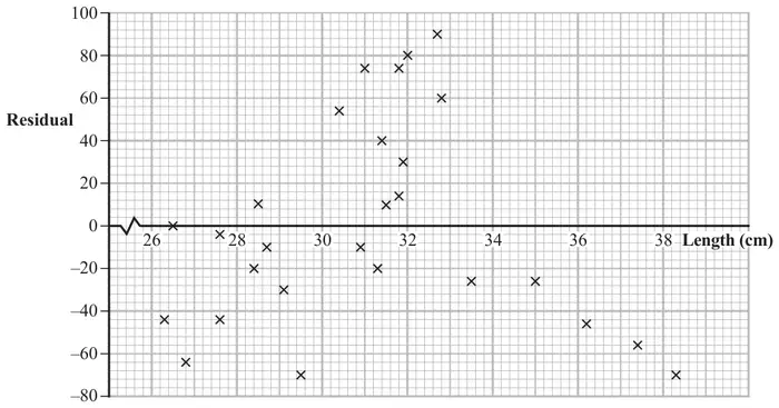
A residual plot for these data is shown below.

Residual plot: residual (from –80 to 100) against length (cm, from 26 to 38) for the 27 bream; the residual at length 32 cm is 80, and all five points with length above 33 cm have negative residuals

One of the bream in the sample has a length of 32 cm.

(d) Find its weight. (2)
(e) With reference to the residual plot, comment on the model for bream with lengths above 33 cm. (1)

A2 June 2022 Q1

EdexcelCurrent spec7 marksCorrelationLinear Regression

1. Kwame is investigating a possible relationship between average March temperature, \(t\,{}^\circ\mathrm{C}\), and tea yield, \(y\) kg/hectare, for tea grown in a particular location.
He uses 30 years of past data to produce the following summary statistics for a linear regression model, with tea yield as the dependent variable.

\[\text{Residual Sum of Squares (RSS)} = 1\,666\,567 \qquad \mathrm{S}_{tt} = 52.0 \qquad \mathrm{S}_{yy} = 1\,774\,155\]\[\text{least squares regression line:} \qquad \text{gradient} = 45.5 \qquad y\text{-intercept} = 2080\]
(a) Use the regression model to predict the tea yield for an average March temperature of \(20\,{}^\circ\mathrm{C}\) (1)

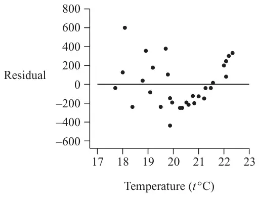
He also produces the following residual plot for the data.

Residual plot: residual (from –600 to 800) against temperature (t °C, from 17 to 23) for the 30 years; residuals are mostly negative between about 20 and 21.5 °C and all positive and rising above 21.5 °C
(b) Explain what you understand by the term residual. (1)
(c) Calculate the product moment correlation coefficient between \(t\) and \(y\) (2)
(d) Explain why the linear model may not be a good fit for the data
(i) with reference to your answer to part (c)
(ii) with reference to the residual plot.
(2)

Kwame also collects data on total March rainfall, \(w\) mm, for each of these 30 years.

For a linear regression model of \(w\) on \(t\) the following summary statistic is found.

\[\text{Residual Sum of Squares (RSS)} = 86\,754\]

Kwame concludes that since this model has a smaller RSS, there must be a stronger linear relationship between \(w\) and \(t\) than between \(y\) and \(t\) (where RSS = 1 666 567)

(e) State, giving a reason, whether or not you agree with the reasoning that led to Kwame’s conclusion. (1)

A2 October 2021 Q4

EdexcelCurrent spec10 marksCorrelationLinear Regression

4. A researcher is investigating the relationship between elevation, \(x\) metres, and annual mean temperature, \(t\,{}^\circ\mathrm{C}\).

From a random sample of 20 weather stations in Switzerland, the following results were obtained

\[\mathrm{S}_{xx} = 8\,820\,655 \qquad \mathrm{S}_{tt} = 444.7 \qquad \sum x = 28\,130 \qquad \sum t = 94.62\]

The product moment correlation coefficient for these data is found to be \(-0.959\)

(a) Interpret the value of this correlation coefficient. (1)
(b) Show that the equation of the regression line of \(t\) on \(x\) can be written as\[t = 14.3 - 0.00681x\] (4)

The random variable \(W\) represents the elevations of the weather stations in kilometres.

(c) Write down the equation of the regression line of \(t\) on \(w\) for these 20 weather stations in the form \(t = a + bw\) (1)
(d) Show that the residual sum of squares (RSS) for the model for \(t\) and \(x\) is 35.7 correct to one decimal place. (1)

One of the weather stations in the sample had a recorded elevation of 1100 metres and an annual mean temperature of \(1.4\,{}^\circ\mathrm{C}\)

(e)
(i) Calculate this weather station’s contribution to the residual sum of squares.
Give your answer as a percentage. (2)
(ii) Comment on the data for this weather station in light of your answer to part (e)(i). (1)

AS October 2020 Q4

EdexcelAS paperCurrent spec14 marksLinear Regression

4. Some students are investigating the strength of wire by suspending a weight at the end of the wire. They measure the diameter of the wire, \(d\) mm, and the weight, \(w\) grams, when the wire fails. Their results are given in the following table.

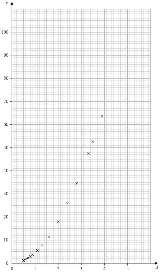
These 14 points are plotted below
\(d\)0.50.60.70.80.91.11.31.62
\(w\)1.21.72.33.03.85.67.711.618
These 14 points are plotted belowNot yet plotted
\(d\)2.42.83.33.53.94.54.64.85.4
\(w\)25.934.947.452.763.98183.689.9109.4

The first 14 points are plotted on the axes on page 13.

Axes for a scatter diagram: w from 0 to 110 against d from 0 to 6, with the first 14 points plotted as crosses, rising steeply in a curve from (0.5, 1.2) to (3.9, 63.9)
(a) On the axes below, complete the scatter diagram for these data. (1)
(b) Use your calculator to write down the equation of the regression line of \(w\) on \(d\). (2)
(c) With reference to the scatter diagram, comment on the appropriateness of using this linear regression model to make predictions for \(w\) for different values of \(d\) between 0.5 and 5.4 (1)

The product moment correlation coefficient for these data is \(r = 0.987\) (to 3 significant figures).

(d) Calculate the residual sum of squares (RSS) for this model. (2)

Robert, one of the students, suggests that the model could be improved and intends to find the equation of the line of regression of \(w\) on \(u\), where \(u = d^2\)
He finds the following statistics

\[\mathrm{S}_{wu} = 5721.625 \qquad \mathrm{S}_{uu} = 1482.619 \qquad \sum u = 157.57\]
(e) By considering the physical nature of the problem, give a reason to support Robert’s suggestion. (1)
(f) Find the equation of the regression line of \(w\) on \(u\). (3)
(g) Find the residual sum of squares (RSS) for Robert’s model. (2)
(h) State, giving a reason based on these calculations, which of these models better describes these data. (1)
(i) Hence estimate the weight at which a piece of wire with diameter 3 mm will fail. (1)

A2 October 2020 Q3

EdexcelCurrent spec6 marksLinear Regression

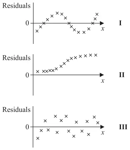
3. Below are 3 sketches from some students of the residuals from their linear regressions of \(y\) on \(x\).

Three residual sketches against x. I: residuals rise above 0, fall below 0, then rise again in a wave pattern. II: all residuals are above 0 and increase steadily. III: residuals scattered randomly above and below 0

For each sketch you should state, giving your reason,

(i) whether or not the sketch is feasible

and if it is feasible

(ii) whether or not the sketch suggests a linear or a non-linear relationship between \(y\) and \(x\). (6)

AS June 2019 Q3

EdexcelAS paperCurrent spec11 marksCorrelationLinear Regression

3. Two students, Jim and Dora, collected data on the mean annual rainfall, \(w\) cm, and the annual yield of leeks, \(l\) tonnes per hectare, for 10 years.

Jim summarised the data as follows

\[\mathrm{S}_{wl} = 42.786 \qquad \mathrm{S}_{ww} = 9936.9 \qquad \sum l^2 = 26.2326 \qquad \sum l = 16.06\]
(a) Find the product moment correlation coefficient between \(l\) and \(w\) (2)

Dora decided to code the data first using \(s = w - 6\) and \(t = l - 20\)

(b) Write down the value of the product moment correlation coefficient between \(s\) and \(t\).
Give a justification for your answer. (1)

Dora calculates the equation of the regression line of \(t\) on \(s\) to be \(t = 0.00431s - 18.87\)

(c) Find the equation of the regression line of \(l\) on \(w\) in the form \(l = a + bw\), giving the values of \(a\) and \(b\) to 3 significant figures. (3)
(d) Use your equation to estimate the yield of leeks when \(w\) is 100 cm. (1)
(e) Calculate the residual sum of squares. (2)

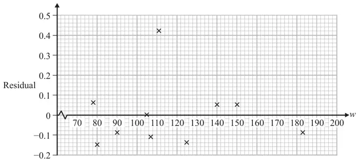
The graph shows the residual for each value of \(l\)

Residual plot: residual (from –0.2 to 0.5) against w (from 70 to 200) for 10 points; one residual of about 0.42 at w = 111, the others between about –0.15 and 0.06
(f)
(i) State whether this graph suggests that the use of a linear regression model is suitable for these data. Give a reason for your answer.
(ii) Other than collecting more data, suggest how to improve the fit of the model in part (c) to the data.
(2)

A2 June 2019 Q2

EdexcelCurrent spec10 marksCorrelationLinear Regression

2. A large field of wheat is split into 8 plots of equal area. Each plot is treated with a different amount of fertiliser, \(f\) grams/m2. The yield of wheat, \(w\) tonnes, from each plot is recorded. The results are summarised below.

\[\sum f = 28 \qquad \sum w = 303 \qquad \sum w^2 = 13\,447 \qquad \mathrm{S}_{ff} = 42 \qquad \mathrm{S}_{fw} = 269.5\]
(a) Calculate the product moment correlation coefficient between \(f\) and \(w\) (2)
(b) Interpret the value of your product moment correlation coefficient. (1)
(c) Find the equation of the regression line of \(w\) on \(f\) in the form \(w = a + bf\) (3)
(d) Using your equation, estimate the decrease in yield when the amount of fertiliser decreases by 0.5 grams/m2 (1)

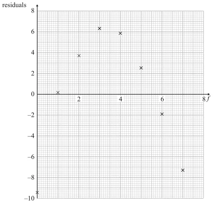
The residuals of the data recorded are calculated and plotted on the graph below.

Graph of residuals (from –10 to 8) against f (from 0 to 8) on a grid: approximately (0, –9.4), (1, 0.2), (2, 3.7), (3, 6.3), (4, 5.9), (5, 2.5), (6, –1.9), (7, –7.3)
(e) With reference to this graph, comment on the suitability of the model you found in part (c). (2)
(f) Suggest how you might be able to refine your model. (1)

AS June 2018 Q1

EdexcelAS paperCurrent spec11 marksCorrelationLinear Regression

1. The scores achieved on a maths test, \(m\), and the scores achieved on a physics test, \(p\), by 16 students are summarised below.

\[\sum m = 392 \qquad \sum p = 254 \qquad \sum p^2 = 4748 \qquad \mathrm{S}_{mm} = 1846 \qquad \mathrm{S}_{mp} = 1115\]
(a) Find the product moment correlation coefficient between \(m\) and \(p\) (2)
(b) Find the equation of the linear regression line of \(p\) on \(m\) (3)

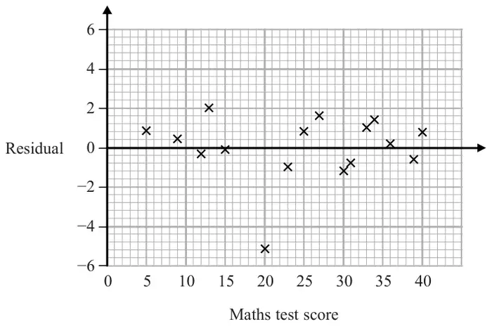
Figure 1 shows a plot of the residuals.

Figure 1: residual (from –6 to 6) against maths test score (from 0 to 40) for 16 students; the point at maths score 20 has residual about –5.1, the others lie between about –1.2 and 2
Figure 1
(c) Calculate the residual sum of squares (RSS). (2)

For the person who scored 30 marks on the maths test,

(d) find the score on the physics test. (2)

The data for the person who scored 20 on the maths test is removed from the data set.

(e) Suggest a reason why. (1)

The product moment correlation coefficient between \(m\) and \(p\) is now recalculated for the remaining 15 students.

(f) Without carrying out any further calculations, suggest how you would expect this recalculated value to compare with your answer to part (a).
Give a reason for your answer. (1)