6. Xiang owns a takeaway restaurant and wants to employ a delivery company. Xiang uses two companies, \(A\) and \(B\), for one week each and records the delivery rate, \(x\) minutes per km, for each delivery.
Company \(A\) made 61 deliveries with \(\bar{x}_A = 3.7\) and \(s_A^{\,2} = 1.64\)
Company \(B\) made 51 deliveries with \(\sum x_B = 142.8\) and \(\sum x_B^{\,2} = 461.34\)
(a) Find unbiased estimates for the mean and variance of the delivery rate for company \(B\). (3)
Xiang wants to carry out a two-sample \(t\)-test to determine whether there is a difference in the mean delivery rate for these companies.
(b) State any assumptions Xiang must make about the delivery rates of the two companies. (1)
(c) Using a 5% level of significance, carry out Xiang’s test. You should clearly state the hypotheses, test statistic and critical value you use. (7)
Xiang noticed that a greater proportion of company \(A\)’s deliveries were in the town, with lots of traffic, whereas a greater proportion of company \(B\)’s deliveries were rural, with less traffic.
Xiang decides to carry out a further test. He selects a random sample of 10 customers who regularly place an order at the same time each week. He asks company \(A\) to deliver these orders one week and company \(B\) the next week. There were no roadworks or other incidents affecting travel time in either week.
The delivery rates are given in the table below.
Customer
1
2
3
4
5
6
7
8
9
10
Company \(A\)
5.4
3.6
2.5
4.7
2.3
3.2
3.4
4.1
5.9
4.5
Company \(B\)
4.9
3.9
2.3
4.5
2.6
2.8
3.1
3.8
5.2
4.3
(d) Use a 5% level of significance to carry out a suitable test to determine whether there is a difference in the delivery rates of the two companies. You should clearly state your hypotheses, test statistic and critical value. (6)
[significant result] there is evidence of a difference in mean delivery rates oe
A1
2.2b
(7)
Notes
1st B1: for correct hypotheses, both in terms of \(\mu\). Can be \(\mu_1\) and \(\mu_2\) etc
1st M1: for correct attempt at \(s_p^{\,2}\) ft their value for \(B\) ;
1st A1: for awrt 1.45 (implied by 2nd A1) \(\left(\frac{1599}{1100}\right)\)
2nd M1: for correct ft expression for test statistic using 3.7 allow (\(\pm\)) standardisation ;
2nd A1: for awrt (\(\pm\)) 3.93 or awrt (\(\pm\)) 3.94
2nd B1: for (\(\pm\))1.982 (or better)
3rd A1:dep on all previous Ms and \(1 \lt |\text{cv}| \lt \) “3.93” for correct conclusion mentioning “mean delivery rate”. Do not allow contradictory statements. Incorrect comparisons A0.
[Not significant] insufficient evidence of a difference in delivery rates oe
A1
2.2b
(6)
(17 marks)
Notes
1st B1: for both hypotheses in terms of \(\mu\) (or \(\mu_d\)) but not \(\mu_1\) and \(\mu_2\) etc
1st M1: for attempting differences (at least 6 correct values) implied by mean or \(s_D^{\,2}\) or \(s_D\)
2nd M: for a correct express’n for \(t\) (ignore df) with their values for \(\bar{x}_D\) and \(s_D\) (correct method)
1st A1: for awrt \(\pm 2.20\) or \(\pm 2.205\) (accept 2.2 if correct expression or \(\bar{x}_D\) and \(s_D\) seen)
2nd B1: for correct cv i.e. \(\pm 2.262\) or better
2nd A1:dep on all previous Ms and “2.20” \(\lt |\text{cv}| \lt 3\) for correct conclusion in context. Do not allow contradictory statements. “mean delivery rate” or incorrect comparison is A0.
SC:If they carry out a \(t\)-test for two independent samples then allow 2nd M1 for standardising with diff of their means and pooled variance and 2nd B1 for cv of \(\pm 2.101\)
4. The weights of apples Sam grows are normally distributed with a mean of 131 g and a standard deviation of 6 g
A supermarket will only buy apples with weights in the range 125 g to 137 g
(a) Find the proportion of apples Sam grows that the supermarket will buy. (1)
Some of Sam’s apple trees are treated with the aim of reducing the variability in weight of apples, without significantly affecting the mean weight. The weights of apples are still normally distributed.
A random sample of 25 apples was taken from treated trees and the weight, \(x\) grams, of each apple was recorded. The results are summarised by the following statistics
(b) Use a 5% level of significance to carry out a suitable test to determine whether there is evidence that the variance of the weights of apples from treated trees has decreased. You should clearly state your test statistic, hypotheses and critical value. (6)
(c) Calculate a 95% confidence interval for the mean weight of apples produced by Sam’s trees after treatment. You should clearly state the formula and numerical expression you have used. (3)
(d)
(i) State, giving a reason, whether the aims of the treatment have been met.
(ii) Give an estimate of the proportion of apples the supermarket will buy from Sam’s trees that have been treated. (3)
5% critical value (lower tail) \(\chi^2_{24}(5\%) = 13.848\)
B1
3.4
(Significant result so reject H0) there is evidence that the treatment works oe orvariance of weights is lower oe
A1
2.2b
(6)
Notes
1st B1: for correct hypotheses in terms of \(\sigma\) or \(\sigma^2\) Do not accept in words.
1st M1: for a correct expression for \(s\) or \(s^2\) Implied by \(\dfrac{181}{12}\) or 15.0833…
2nd M1: for a correct expression for ts (ft their 15.0833…) May be implied by awrt 10.1
1st A1: for awrt 10.1 or may see \(\dfrac{181}{18}\)
2nd B1: for the correct cv of 13.848 (accept 13.8 or better or allow 13.85)
2nd A1: for a correct conclusion in context (independent of hypotheses but dep on M2 and their ts < cv where 12 < cv < 15). Incorrect comparison or contradictory statement is A0
M1: for an attempt at a correct formula with 130 or their 3.88… and \(\sqrt{25}\) and \(t \gt 2\)
1st A1ft: for a correct expression using \(t = 2.064\) (or better) can ft their 3.88… = their \(s\)
2nd A1: for awrt (128, 132) provided M1 clearly scored.
Mark scheme (d)
Scheme
Marks
AO
(i) Yes (or treatment worked) since 131 is in CI (and \(\sigma\) reduced)
B1
2.4
(ii) Assume \(\sigma = \) “3.9” (or better) and suitable \(\mu\) e.g. 131
M1
3.5a
Proportion in range (79% ~ 88%)
A1
1.1b
(3)
(13 marks)
Notes
(i) B1: dep on a CI in (c) which includes 131 and concluding variance lower in (b). For stating treatment was successful (o.e. condone e.g. yes) and mentioning 131 (or referred to as the mean) is inside CI. Do not allow reference to critical region for CI.
(ii) M1: for evidence of a suitable \(\sigma\) used (ft their \(s\)) and a value of \(\mu\) from their CI. Must see their values for \(\mu\) and \(\sigma\) to score.
A1: dep on \(\sigma\) = awrt 3.9 and \(\mu = [\text{awrt}\,128,\ \text{awrt}\,132]\) for an answer in the range 0.79 to 0.88 inclusive (decimal or %)
3. A scientist investigated the effects of nitrogen-fixing bacteria on cereal crop yield, \(x\,\mathrm{kg\,ha^{-1}}\)
The data come from independent random samples from normal distributions.
The results are summarised in the table below.
\(n\)
\(\bar{x}\)
\(s_x\)
Without nitrogen-fixing bacteria
6
1648
143.8
With nitrogen-fixing bacteria
5
1910
64.0
(a) Test whether or not the variances of the cereal crop yields are the same. You should use a 10% level of significance and state your hypotheses and critical value clearly. (4)
A suitable test to determine whether there is an increase in mean cereal crop yield has a \(p\)-value of 0.002
(b)
(i) Explain the importance of the conclusion of the test in part (a) to this test.
(ii) Comment on the effectiveness of nitrogen-fixing bacteria on cereal crop yields. (2)
(Not significant) insufficient evidence of a difference in variances
A1
2.2b
(4)
Notes
B1: for both hypotheses correct in terms of \(\sigma\) or \(\sigma^2\) May use labelling of e.g. 1 and 2 or e.g. “with” and “without”. Condone \(x\) and \(y\).
M1: for a correct numerical expression for \(F\) (must have squares but does not need to be evaluated) May be implied by awrt 5.05 Could be reciprocal.
B1: for 6.26 (or better) If reciprocal (0.198…) is used as test statistic then need \(\dfrac{1}{5.19}\) or awrt 0.193
A1: dep on a critical value such that awrt \(5.05 \lt \text{cv} \lt 7\) for a correct test statistic awrt 5.05, and correct conclusion. Condone e.g. variances are the same. Do not accept conclusions which do not refer to the variances. If an incorrect comparison or statement is made A0
Mark scheme (b)
Scheme
Marks
AO
(i) Need to assume variances are the same to carry out the test for means (the test showed that the variances could be assumed to be equal)
B1
2.4
(ii) There is evidence it increases mean yield (but does not effect variance)
B1
2.2b
(2)
(6 marks)
Notes
(i) B1: for recognising that the test (for difference of means) requires the populations to have the same variance oe. Must indicate that it is a requirement (not just that you can assume the variances are equal). Must be in words. Allow explanations suggesting that it enables a pooled estimate for \(\sigma^2\) or a better estimate of \(\sigma^2\) to be found (so that a \(t\)-test can be carried out on the difference between means of two independent distributions with unknown variances) Do not allow references to the normal distribution being used.
(ii) B1: for a correct conclusion in context mentioning increase in mean yield. Does not require the comment about variances.
6. A researcher set up a trial to assess the effect that a food supplement has on the increase in weight of Herdwick lambs. The researcher randomly selected 8 sets of twin lambs. One of each set of twins was given the food supplement and the other had no food supplement. The gain in weight, in kg, of each lamb over the period of the trial was recorded.
Set of twin lambs
\(A\)
\(B\)
\(C\)
\(D\)
\(E\)
\(F\)
\(G\)
\(H\)
Weight gain (kg)
With food supplement
4.1
5.3
6.0
3.6
5.9
4.2
7.1
6.4
No food supplement
5.0
4.8
5.2
3.4
5.1
3.9
7.0
6.5
(a) State why a two sample \(t\)-test is not suitable for use with these data. (1)
(b) Suggest 2 other factors about the lambs that the researcher may need to control when selecting the sample. (2)
(c) State one assumption, in context, that needs to be made for a paired \(t\)-test to be valid. (1)
For a pair of twin lambs, the random variable \(W\) represents the weight gain of the lamb given the food supplement minus the weight gain of the lamb not given the food supplement.
(d) Using the data in the table, calculate a 98% confidence interval for the mean of \(W\) Show your working clearly. (5)
The researcher believes that the mean of \(W\) is greater than 200 g
(e) Stating your hypotheses clearly, use your confidence interval to explain whether or not there is evidence to support the researcher’s belief. (3)
Mark scheme (a)
Scheme
Marks
AO
The samples are not independent
B1
3.5b
(1)
Notes
B1: The idea that samples are not independent. Condone other irrelevant comments provided they do not contradict this.
Mark scheme (b)
Scheme
Marks
AO
They should consider the birth weight, gender, or whether or not the lambs are premature. oe
B1 B1
2.4 2.4
(2)
Notes
B1: For one suitable comment on twins being identical relating to selecting the sample. Condone start weight. Do not accept age / diets of the lambs
B1: For a second suitable comment.
Mark scheme (c)
Scheme
Marks
AO
Need the assumption that the underlying distribution of the difference between the weight gains must be normally distributed.
M1: attempting differences (at least 4 correct) implied by awrt 0.304 or 0.551 but not 0.2125
M1: attempt to find \(\bar{w}\) and \(s\) or \(s^2\) for their differences implied by 0.2125 and either awrt 0.304 or 0.551
M1: For using the correct formula their \(\bar{w} \pm t \times \sqrt{\dfrac{\text{their } s^2}{8}}\) where \(|t| \gt 2\) all values need to be substituted in.
A1ft: for their \(\bar{w} \pm\) awrt \(2.998 \times \sqrt{\dfrac{\text{their } s^2}{8}}\) all values need to be substituted in
A1: dependent on all previous method marks (awrt -0.372, awrt 0.797)
SC: If they have carried out a CI for two independent samples allow 3rd M for using their difference of their means and a pooled variance and A1ft using correct formula with awrt 2.624
There is no evidence that \(\mu_w\) is greater than 0.2 oe
A1ft
2.2b
(3)
(12 marks)
Notes
B1: For both hypotheses correct in terms of \(\mu\) or \(\mu_w\) Condone 200
M1: For changing 200 g to 0.2 kg (ignore units for this mark) and comparing to their CI
A1ft: Independent of hypotheses. Drawing a correct inference following through on their CI provided 0.2 is within their confidence interval, with no contradictory statements. Does not need to be in context. Accept “insufficient evidence to support the (researcher’s) belief”.
3. A factory produces bolts. The lengths of the bolts are normally distributed with mean \(\mu\) mm and standard deviation 0.868 mm
A random sample of 15 of these bolts is taken and the mean length is 30.03 mm
(a) Calculate a 90% confidence interval for \(\mu\) (3)
A suitable test, at the 10% level of significance, is carried out using these 15 bolts, to see whether or not there is evidence that the variance of the length of the bolts has increased.
(b) Calculate the critical region for \(S^2\) (3)
The manager of the factory decides that, in future, he will check each month whether the machine making the bolts is working properly. He uses a 10% level of significance to test whether or not there is evidence that
the mean length of the bolts has changed
the variance of the length of the bolts has increased
The next month a random sample of 15 bolts is taken.
The mean length of these bolts is 30.06 mm and the standard deviation is 1.02 mm
(c) With reference to your answers to part (a) and part (b), state whether or not there is any evidence that the machine is not working properly. Give reasons for your answer. (2)
B1: For realising a chi squared distribution must be used as a model and CV = awrt 21.06
M1: Correct method comparing \(\dfrac{14S^2}{0.868^2}\) to \(19 \lt \chi^2_{14} \lt 24\) (condone equals instead of >) Ignore any additional calculations outside of this range.
A1: Correct CR allow awrt 1.13 only
Mark scheme (c)
Scheme
Marks
AO
Insufficient evidence that the machine is not working properly as 30.06 is within the confidence interval
M1
2.2b
and 1.022 (1.0404) is not in the CR oe
A1ft
2.4
(2)
(8 marks)
Notes
M1:Dependent on an answer to part (a) or part (b) in order to draw an inference. Drawing a correct inference that there is insufficient evidence to suggest that the machine is not working properly following through one of their CR or CI with one correct comparison. Must mention the machine at least once. If they have either 30.06 outside their CI or 1.022 in their CR then allow an inference that the machine is not working properly for this mark following a correct comparison and no contradictory statements relating to that comparison. This mark can still be scored if there is a second comparison which is incorrect.
A1ft:Dependent on 30.06 in their confidence interval and 1.022 not in the CR. For drawing a correct inference following through their CR or CI with both correct comparisons and no contradictory statements. Must mention the machine at least once. Do not accept a comparison of 30.06 with just one of the limits for the CI.
5. A psychologist claims to have developed a technique to improve a person’s memory.
A random sample of 8 people are each given the same list of words to memorise and recall.
Each person then receives memory training from the psychologist. After the training, each person is given the same list of new words to memorise and recall.
The table shows the percentage of words recalled by each person before and after the training.
Person
\(A\)
\(B\)
\(C\)
\(D\)
\(E\)
\(F\)
\(G\)
\(H\)
Percentage of words recalled before training
24
33
33
39
30
38
32
34
Percentage of words recalled after training
28
30
37
41
32
44
35
34
(a) State why a paired \(t\)-test is suitable for these data. (1)
(b) State an assumption that needs to be made in order to carry out a paired \(t\)-test in this case. (1)
(c) Test, at the 5% level of significance, whether or not there is evidence of an increase in the percentage of words recalled after receiving the psychologist’s training. State your hypotheses, test statistic and critical value used for this test. (7)
Mark scheme (a)
Scheme
Marks
AO
e.g. for each person the scores before and after are not independent
B1
2.4
(1)
Notes
B1: correct explanation
Mark scheme (b)
Scheme
Marks
AO
The differences in scores are normally distributed.
2.30 > 1.895, therefore (reject H0) there is sufficient evidence to: support an increase in the percentage of words recalled or support psychologist’s claim
A1ft
2.2b
(7)
(9 marks)
Notes
M1: for setting up paired \(t\)-test with at least 5 correct differences consistent in direction
M1: complete method for \(\bar{d}\) and \(s_\mathrm{d}\) or \(s_d^{\,2}\)
B1: Use of \(t\)-distribution for differences with both hypotheses correct in terms of \(\mu\) / \(\mu_\mathrm{d}\) Allow \(\mu_\mathrm{d} \lt 0\) if candidate does test with negative test statistic
M1: method for finding test statistic with their values
A1: awrt \(\pm\)2.30
B1: correct critical \(\pm\)1.895 (or better) with compatible sign
A1ft: drawing a correct inference in context Must be consistent with their CV and a standardised test statistic from \(t\)-distribution Must mention “percentage” and “words” or “psychologist’s claim”
SC: If they have carried out a \(t\)-test for two independent samples they can potentially score: M0M0B0M1A0B1A1ft If they do follow this path, they can score: 3rd M1 for standardising with difference of their means and a pooled variance 2nd B1 for a CV of 1.761 A1ft for a correct contextual conclusion for their test statistic and 1.761
3. Two machines, \(A\) and \(B\), are used to fill bottles of water. The amount of water dispensed by each machine is normally distributed.
Samples are taken from each machine and the amount of water, \(x\) ml, dispensed in each bottle is recorded. The table shows the summary statistics for Machine \(A\).
Sample size
\(\sum x\)
\(\sum x^2\)
Machine \(A\)
9
2268
571 700
(a) Find a 95% confidence interval for the variance of the amount of water dispensed in each bottle by Machine \(A\). (4)
For Machine \(B\), a random sample of 11 bottles is taken. The sample variance of the amount of water dispensed in bottles is 12.7 ml2
(b) Test, at the 10% level of significance, whether there is evidence that the variances of the amounts of water dispensed in bottles by the two machines are different. You should state the hypotheses and the critical value used. (4)
There is insufficient evidence to suggest that the variances are different.
A1
2.2b
(4)
(8 marks)
Notes
B1: both hypotheses correct using \(\sigma\) or \(\sigma^2\)
M1: using the \(F\)-distribution as the model eg \(\dfrac{s_A^2}{s_B^2}\)
B1: awrt 3.07
A1: Drawing a correct inference following through their CV and value for Allow \(\sigma_B^2 = \sigma_A^2\) Allow standard deviation instead of variance
NB: Allow candidates to use their \(\dfrac{s_B^2}{s_A^2}\) with \(\dfrac{1}{3.35}\) = awrt 0.299 for the final M1B1A1 in (b)
2. Camilo grows two types of apple, green apples and red apples.
The standard deviation of the weights of green apples is known to be 3.5 grams.
A random sample of 80 green apples has a mean weight of 128 grams.
(a) Find a 98% confidence interval for the mean weight of the population of green apples. Show your working clearly and give the confidence interval limits to 2 decimal places. (3)
Camilo believes that the mean weight of the population of green apples is more than 10 grams greater than the mean weight of the population of red apples.
A random sample of \(n\) red apples has a mean weight of 117 grams.
The standard deviation of the weights of the red apples is known to be 4 grams.
A test of Camilo’s belief is carried out at the 5% level of significance.
(b) State the null and alternative hypotheses for this test. (1)
(c) Find the smallest value of \(n\) for which the null hypothesis will be rejected. (6)
(d) Explain the relevance of the Central Limit Theorem in parts (a) and (c). (1)
(e) Given that \(n = 85\), state the conclusion of the hypothesis test. (1)
Mark scheme (a)
Scheme
Marks
AO
\(z = 2.3263\)
B1
1.1b
98% CI for \(\mu\) is: \(128 \pm 2.3263 \times \dfrac{3.5}{\sqrt{80}}\)
M1: setting up normal model with correct mean or variance May be shown in standardisation with correct mean or variance and \(|z| \gt 1\)
A1: correct variance and mean, may be seen in standardisation
M1: setting up an equation or inequality by standardising with their mean and their standard deviation and \(|z| \gt 1\)
B1: Correct critical value 1.6449 or better, allow 1.64 or better
M1: rearranging to solve for \(n\) (may be implied by 73.9…)
A1: \(n = 74\) cao
Mark scheme (d)
Scheme
Marks
AO
Sample sizes are large so CLT means even though we do not know the distributions of \(G\) and \(R\), the means \(\bar{G}\) and \(\bar{G} - \bar{R}\) will be (approximately) normally distributed.
B1
2.4
(1)
Notes
B1: correct explanation mentioning large sample size and the means being distributed normally
Mark scheme (e)
Scheme
Marks
AO
[Since 85 > 73.9…] there is significant evidence to support Camilo’s belief/the mean weight of green apples is more than 10 grams greater than red apples is supported.
B1ft
2.2b
(1)
(12 marks)
Notes
B1ft: drawing a correct inference in context, must be consistent with their value of \(n\)
5. The concentration of an air pollutant is measured in micrograms/m3
Samples of air were taken at two different sites and the concentration of this particular air pollutant was recorded.
For Site \(A\) the summary statistics are shown below.
number of samples
\(s_A^2\)
Site \(A\)
13
6.39
For Site \(B\) there were 9 samples of air taken.
A test of the hypothesis \(\mathrm{H}_0 : \sigma_A^2 = \sigma_B^2\) against the hypothesis \(\mathrm{H}_1 : \sigma_A^2 \neq \sigma_B^2\) is carried out using a 2% level of significance.
(a) State a necessary assumption required to carry out the test. (1)
Given that the assumption in part (a) holds,
(b) find the set of values of \(s_B^2\) that would lead to the null hypothesis being rejected, (4)
(c) find a 99% confidence interval for the variance of the concentration of the air pollutant at Site \(\boldsymbol{A}\). (3)
Mark scheme (a)
Scheme
Marks
AO
The concentration of air pollutant (for each site) follows a normal distribution
B1
2.4
(1)
Notes
B1: Correct modelling assumption. Allow air pollutant samples are independent. Samples of air pollutant are normally distributed is B0
M1: For realising a \(\chi^2\) distribution must be used as a model with at least one value correct. Allow \(\chi^2_{12,\,0.01} = 26.217\) or \(\chi^2_{12,\,0.99} = 3.571\) for this mark.
4. A doctor believes that a four-week exercise programme can reduce the resting heart rate of her patients. She takes a random sample of 7 patients and records their resting heart rate before the exercise programme and again after the exercise programme.
Patient
\(A\)
\(B\)
\(C\)
\(D\)
\(E\)
\(F\)
\(G\)
Resting heart rate before
65
68
77
79
80
88
92
Resting heart rate after
63
65
73
76
80
84
80
(a) Using a 5% level of significance, carry out an appropriate test of the doctor’s belief. You should state your hypotheses, test statistic and critical value. (7)
(b) State the assumption made about the resting heart rates that was required to carry out the test. (1)
[\(2.80 \gt 1.943\),] therefore there is sufficient evidence to support the doctor’s belief/evidence to suggest resting heart rate is reduced.
A1
2.2b
(7)
Notes
M1: For understanding paired \(t\)-test is required and attempting to find differences at least 5 correct, allow \(\pm\) (may be implied by correct \(\bar{d}\) and \(s_\mathrm{d}\))
M1: Complete method for \(\bar{d}\) and \(s_\mathrm{d}\) or \((s_\mathrm{d})^2\)
B1: Correct model for differences with both hypotheses correct in terms of \(\mu\) / \(\mu_\mathrm{d}\) (sign of \(\mathrm{H}_1\) must be compatible with their \(\bar{d}\))
M1: Method for finding test statistic with their values
B1: Correct critical \(\pm 1.943\) (or better) with compatible sign
A1: Correct comparison to deduce that the doctor’s belief is supported. Must be consistent with their CV and their test statistic (dependent upon all M marks).
SC: Difference of means test apply scheme but also allow 2nd B1 for \(t_{12} = 1.782\)
Mark scheme (b)
Scheme
Marks
AO
Differences in resting heart rates must be normally distributed for the test to be valid.
2. A factory produces yellow tennis balls and white tennis balls. Independent samples, one of yellow tennis balls and one of white tennis balls, are taken. The table shows information about the weights of the yellow tennis balls, \(Y\) grams, and the weights of the white tennis balls, \(W\) grams.
Sample size
Mean weight of random sample (grams)
Known population standard deviation of weights (grams)
Yellow tennis balls
120
57.2
1.2
White tennis balls
140
56.9
0.9
(a) Find a 95% confidence interval for the mean weight of yellow tennis balls. (3)
Jamie claims that the mean weight of the population of yellow tennis balls is greater than the mean weight of the population of white tennis balls. A test of Jamie’s claim is carried out.
(b)
(i) Specify the approximate distribution of \(\overline{Y} - \overline{W}\) under the null hypothesis of the test. (3)
(ii) Explain the relevance of the large sample sizes to your answer to part (i). (1)
(c) Complete the hypothesis test using a 5% level of significance. You should state your hypotheses and the value of your test statistic clearly. (5)
(ii) Central limit theorem applies so we do not need to know the distributions of \(Y\) and \(W\)/ Allows us to assume that sample means (\(\overline{Y}\) and \(\overline{W}\)) are normally distributed.
B1
2.4
(1)
Notes
M1: Translating context into a Normal distribution model
A1: Correct mean
A1: Correct variance (allow awrt 0.0178 or exact fraction \(\dfrac{249}{14000}\))
B1: Correct explanation about the distributions of \(Y\) and \(W\) or \(\overline{Y}\) and \(\overline{W}\)
[Reject \(\mathrm{H}_0\)] Significant evidence to support Jamie’s claim/mean weight of the population of yellow tennis balls is greater than mean weight of the population of white tennis balls.
A1
2.2b
(5)
(12 marks)
Notes
B1: Both hypotheses (oe) correct with correct notation (if using \(\mu_x\) and \(\mu_y\) these must be defined).
M1: Standardising using normal distribution test statistic for difference of two means with known variance
A1: awrt 2.25
B1: Correct critical value 1.6449 or better, [or \(p\) = 0.01 or better from correct working]
A1: Drawing a correct inference in context. Do not allow contradictory statements, e.g. ‘Do not reject \(\mathrm{H}_0\), so Jamie’s claim is supported’
6. Elsa is collecting information on the wingspan of two different species of butterfly, Ringlet and Meadow Brown. She takes a random sample of each type of butterfly. The wingspans, \(w\) cm, are summarised in the table below. The wingspans of Ringlet and Meadow Brown butterflies each follow normal distributions.
Number of butterflies
\(\sum w\)
\(\sum w^2\)
Ringlet
8
410
21 032
Meadow Brown
6
294
14 426
(a) Test, at the 2% level of significance, whether or not there is evidence that the variance of the wingspans of Ringlet butterflies is different from the variance of the wingspans of Meadow Brown butterflies. You should state your hypotheses clearly. (7)
The \(k\)% confidence interval for the variance of the wingspans of Meadow Brown butterflies is (1.194, 48.54)
(b) Find the value of \(k\) (3)
(c) Calculate a 95% confidence interval for the difference between the mean wingspan of the Ringlet butterfly and the mean wingspan of the Meadow Brown butterfly. (5)
2. A company produces two colours of candles, blue and white. The standard deviation of the burning times of the blue candles is 2.6 minutes and the standard deviation of the burning times of the white candles is 2.4 minutes.
Nissim claims that the mean burning time of blue candles is more than 5 minutes greater than the mean burning time of white candles.
A random sample of 90 blue candles is found to have a mean burning time of 39.5 minutes. A random sample of 80 white candles is found to have a mean burning time of 33.7 minutes.
(a) Stating your hypotheses clearly, use a suitable test to assess Nissim’s belief. Use a 1% level of significance. (6)
(b) Explain how the hypothesis test in part (a) would be carried out differently if the variances of the burning times of candles were unknown. (1)
The burning times for the candles may not follow a normal distribution.
(c) Describe the effect this would have on the calculations in the hypothesis test in part (a). Give a reason for your answer. (2)
6. A new employee, Kim, joins an existing employee, Jiang, to work in the quality control department of a company producing steel rods. Each day a random sample of rods is taken, their lengths measured and a 95% confidence interval for the mean length of the rods, in metres, is calculated. It is assumed that the lengths of the rods produced are normally distributed.
Kim took a random sample of 25 rods and used the \(t\) distribution to obtain a 95% confidence interval of (1.193, 1.367) for the mean length of the rods. Jiang commented that this interval was a little wider than usual and explained that they usually assume that the standard deviation does not change and can be taken as 0.175 metres.
(a) Test, at the 10% level of significance, whether or not Kim’s sample suggests that the standard deviation is different from 0.175 metres. State your hypotheses clearly. (9)
Using Kim’s sample and the normal distribution with a standard deviation of 0.175 metres,
(b) find a 95% confidence interval for the mean length of the rods. (3)
Mark scheme (a)
Scheme
Marks
AO
From CI \(\bar{x} = \dfrac{1.193 + 1.367}{2} = 1.28\) or width = 1.367 – 1.193 = 0.174
1. Gina receives a large number of packages from two companies, \(A\) and \(B\). She believes that the variance of the weights of packages from company \(A\) is greater than the variance of the weights of packages from company \(B\).
Gina takes a random sample of 7 packages from company \(A\) and an independent random sample of 10 packages from company \(B\). Her results are summarised below
Significant, there is evidence to support Gina’s belief
A1
2.2b
(6)
(6 marks)
Notes
1st B1 for both hypotheses in terms of \(\sigma\).
1st M1 for at least one of the \(s^2\) calculations correctly attempted NB \(s_a = 155.72\ldots\) accept awrt 156 and \(s_b = 79.137\ldots\) accept awrt 79.1
2nd M1 for a correct calculation of the test statistic (ft their \(s^2\))
1st A1 for awrt 3.87
2nd B1 for correct cv awrt 3.37
2nd A1 for a correct conclusion mentioning Gina’s belief (o.e.)
6. A company manufactures bolts. The diameter of the bolts follows a normal distribution with a mean diameter of 5 mm.
Stan believes that the mean diameter of the bolts is less than 5 mm. He takes a random sample of 10 bolts and measures their diameters. He calculates some statistics but spills ink on his work before completing them. The only information he has left is as follows
Stating your hypotheses clearly, test, at the 5% level of significance, whether or not Stan’s belief is supported. (9)
Mark scheme
Scheme
Marks
AO
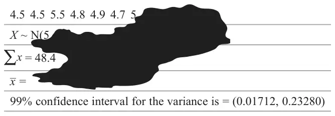
99% confidence interval for Var uses \(\chi^2\) values of 1.735 or 23.589
Stan’s belief is supported or there is evidence that the mean diameter of the bolts is less than 5mm
A1ft
2.2b
(9)
(9 marks)
Notes
B1: For realising a \(\chi^2\) distribution must be used as a model and finding a correct value
M1: For realising the need to set \(\dfrac{9s^2}{\text{“}\text{smallest } \chi^2\text{”}} = 0.2328\) or \(\dfrac{9s^2}{\text{“}\text{largest } \chi^2\text{”}} = 0.01712\)
dM1: correct method used to solve equation to find \(s^2\)
B1: awrt 4.84
B1: Both hypotheses correct using the notation \(\mu\)
B1: \(\pm\) 1.833
M1: For us of correct formula ie \(\pm\dfrac{\text{“}\text{their } 4.84\text{”} - 5}{\sqrt{\text{“}\text{their } 0.0449\text{”}/10}}\) If “4.84” not shown it must be correct here
A1: \(-2.39\)
A1ft: Drawing a correct inference following through their CV and test statistic (must have matching signs)
NB if chi squared values not shown \(s^2 = 0.045\) or 0.0449 award B0 M1M1 for awrt 0.04487 award B1 M1 A1
Use of \(2(2.5758)\dfrac{\sigma}{\sqrt{10}} = 0.21568\) gives \(\sigma = \sqrt{0.0175}\) could get B0M0M0B1B1B1M0A0A0 Unless continue to get \(s^2 = \dfrac{10}{9}0.0175 = 0.0194\ldots\)
Use of \(2(1.833)\dfrac{s}{\sqrt{10}} = 0.21568\) gives \(s = 0.1860\) could get B0M0M0B1B1B1M1A0A1
5. Alexa believes that students are equally likely to achieve the same percentage score on each of two tests, paper I and paper II. She randomly selects 8 students and gives them each paper I and paper II. The percentage scores for each paper are recorded.
The following paired data are collected.
Student
\(A\)
\(B\)
\(C\)
\(D\)
\(E\)
\(F\)
\(G\)
\(H\)
Paper I (%)
70
70
84
80
64
65
65
90
Paper II (%)
64
76
72
74
68
64
58
76
Test, at the 1% significance level, whether or not there is evidence to support Alexa’s belief. State your hypotheses clearly and show your working. (7)
There is insufficient evidence that the papers are of a different level of difficulty or Alexa’s belief is correct
A1ft
2.2b
(7)
(7 marks)
Notes
M1: for realising that the model to use is the paired \(t\)-test and finding the differences \((\pm)\) At least 3 correct
M1: correct method for finding \(\bar{d}\) and \(s_\mathrm{d}\).
B1: Using a correct model for difference and both hypotheses correct using the notation \(\mu_\mathrm{d}\) or \(\mu\) Condone \(\mu_I = \mu_{II}\) and \(\mu_I \neq \mu_{II}\)
M1: Using the correct method to find test statistics ie \(t = \pm\dfrac{\text{“}\text{their } 4.5\text{”}\sqrt{8}}{\text{“}\text{their } 7.09\ldots\text{”}}\)
A1: awrt 1.79 or 1.8
B1: for correct critical value \(t = \pm 3.499\) with compatible sign
A1ft: Drawing a correct inference in context using their CV and their value of \(t\)
3. Yin grows two varieties of potato, plant \(A\) and plant \(B\). A random sample of each variety of potato is taken and the yield, \(x\) kg, produced by each plant is measured. The following statistics are obtained from the data.
Number of plants
\(\sum x\)
\(\sum x^2\)
\(A\)
25
194.7
1637.37
\(B\)
26
227.5
2031.19
(a) Stating your hypotheses clearly, test, at the 10% significance level, whether or not the variances of the yields of the two varieties of potato are the same. (7)
(b) State an assumption you have made in order to carry out the test in part (a). (1)
There is evidence that the two variances are different.
A1ft
2.2b
(7)
Notes
B1: both hypotheses correct using \(\sigma\) or \(\sigma^2\)
M1: Using a correct method for either \(s_A^2\) or \(s_B^2\). May be implied by a correct value
A1: awrt 5.04
A1: awrt 1.62
M1: Using the F-distribution as the model eg \(\dfrac{s_A^2}{s_B^2}\) \(\left(\text{allow } \dfrac{s_B^2}{s_A^2}[= 0.321\ldots]\right)\)
B1: awrt 1.96 or 0.506 must match their method
A1ft: Drawing a correct inference following through their CV and value for \(\dfrac{s_B^2}{s_A^2}\) or \(\dfrac{s_A^2}{s_B^2}\) Allow \(\sigma_B^2 \neq \sigma_A^2\) Allow standard deviation instead of Var. Do not allow \(\sigma_B^2 = \sigma_A^2\)
Mark scheme (b)
Scheme
Marks
AO
The yields are normally distributed.
B1
1.2
(1)
(8 marks)
Notes
B1: recalling the fact that the variable yield needs to be normally distributed
4. A glue supplier claims that Goglue is stronger than Tackfast. A company is presently using Tackfast but agrees to change to Goglue if, at the 5% significance level,
the standard deviation of the force required for Goglue to fail is not greater than the standard deviation of the force required for Tackfast to fail and
the mean force required for Goglue to fail is more than 4 newtons greater than the mean force for Tackfast to fail.
A series of trials is carried out, using Goglue and Tackfast, and the glues are tested to destruction. The force, \(x\) newtons, at which each glue fails is recorded.
Sample size (\(n\))
Sample mean (\(\bar{x}\))
Standard deviation (\(s\))
Tackfast (\(T\))
6
5.27
0.31
Goglue (\(G\))
5
10.12
0.66
It can be assumed that the force at which each glue fails is normally distributed.
(a) Test, at the 5% level of significance, whether or not there is evidence that the standard deviation of the force required for Goglue to fail is greater than the standard deviation of the force required for the Tackfast to fail. State your hypotheses clearly. (5)
The supplier claims that the mean force required for its Goglue to fail is more than 4 newtons greater than the mean force required for Tackfast to fail.
(b) Stating your hypotheses clearly and using a 5% level of significance, test the supplier’s claim. (7)
(c) Show that, at the 5% level of significance, the supplier’s claim will be accepted if \(\bar{X}_G - \bar{X}_T \gt 4.55\), where \(\bar{X}_G\) and \(\bar{X}_T\) are the mean forces required for Goglue to fail and Tackfast to fail respectively. (2)
Later, it was found that an error had been made when recording the results for Goglue. This resulted in all the forces recorded for Goglue being 0.5 newtons more than they should have been. The results for Tackfast were correct.
(d) Explain whether or not this information affects the decision about which glue the supplier decides to use. (3)
Not in critical region, therefore no evidence to reject \(\mathrm{H}_0\)
No evidence of difference in standard deviation (allow variance)
A1cso
(5)
Notes
B1 both hypotheses. allow \(\mathrm{H}_0 : \sigma_T = \sigma_G\) against \(\mathrm{H}_1 : \sigma_G \gt \sigma_T\). Must use \(\sigma\) or \(\sigma^2\) and make clear which is \(\mathrm{H}_0\) and which is \(\mathrm{H}_1\). Do not allow in words
M1 allow 0.31 and 0.66 rather than 0.312 and 0.662 if they write the formula down
B1 correct CV for their \(F\) or a correct comparison if use \(p\)
Final A1: – All previous marks must be awarded. Variances are the same or var are not different
There is evidence to reject \(\mathrm{H}_0\) \(\mu_G\) is greater than \(\mu_T + 4\). The suppliers claim is supported.
A1
(7)
Notes
M1 Allow use of 0.31 and 0.66. May be seen in part (a)
B1 both hypotheses using \(\mu\). Do not allow \(\geqslant\) sign instead of >. May use different letters eg \(A\) and \(B\) but they must be defined.
B1 correct CV but must match \(t\)-value or a correct comparison if use \(p\)
M1 use of correct formula with their \(s_p\) – condone missing 4
M1 use of correct formula with their \(s_p\). (which must have been attempted)
A1 A correct statement or longhand of suppliers claim with the word force and mean and is more than 4 greater oe Do not allow contradicting statements.
M1 correct LHS with 1.833 ( or their CV used in (b)) NB subst in 4.55 for is M0
Mark scheme (d)
Scheme
Marks
No change to standard deviation
B1
\(\bar{X}_G - \bar{X}_T = 4.35\)
M1
Previously they would have changed to Goglue, now they will remain with Tackfast or they will no longer change, or they would have changed but now they will not oe
3. A random sample of 8 students is selected from a school database.
Each student’s reaction time is measured at the start of the school day and again at the end of the school day. The reaction times, in milliseconds, are recorded below.
Student
\(A\)
\(B\)
\(C\)
\(D\)
\(E\)
\(F\)
\(G\)
\(H\)
Reaction time at the start of the school day
10.8
7.2
8.7
6.8
9.4
10.9
11.1
7.6
Reaction time at the end of the school day
10
6.1
8.8
5.7
8.7
8.1
9.8
6.8
(a) State one assumption that needs to be made in order to carry out a paired \(t\)-test. (1)
The random variable \(R\) is the reaction time at the start of the school day minus the reaction time at the end of the school day. The mean of \(R\) is \(\mu\).
John uses a paired \(t\)-test to test the hypotheses
2. Merchandise is sold at concerts. The manager of a concert claims that the mean value of merchandise sold to premium ticket holders is more than £6 greater than the mean value of merchandise sold to standard ticket holders.
(a) Given that all the tickets for the next concert have been sold, describe how a stratified sample should be taken at the concert. (3)
The mean value of merchandise sold to a random sample of 60 standard ticket holders at the concert is £15 with a standard deviation of £10.
The mean value of merchandise sold to a random sample of 55 premium ticket holders at the concert is £23 with a standard deviation of £8.
(b) Test the manager’s claim at the 5% level of significance. State your hypotheses clearly. (8)
(c) For the test in part (b), state whether or not it is necessary to assume that values of merchandise sold have normal distributions. Give a reason for your answer. (2)
Mark scheme (a)
Scheme
Marks
Record / List all ticket numbers of standard and premium tickets
B1
Use random numbers to select a sample of standard and a sample of premium ticket holders i.e. within strata.
B1
Sample sizes in proportion to the no of standard and no of premium ticket holders at the concert.
B1
(3)
Notes
1st B1 Sampling frame in context. Accept list of all standard and premium ticket holders at the concert.
2nd B1 Use of random selection eg simple random sampling within strata
Not significant, insufficient evidence to reject \(\mathrm{H}_0\)
dM1
Insufficient evidence to support the manager’s claim or the mean value of merchandise sold to premium ticket holders is NOT more than £6 greater than the mean value of merchandise sold to standard ticket holders.
A1cso
(8)
Notes
1st & 2nd B1 for hypotheses. Accept \(\mu_1, \mu_2\) or \(\mu_A, \mu_B\) etc if it is clear which is which.
1st M1 for an attempt at se with 3 out of 4 values correct.
Condone switching 10 and 8: \(\sqrt{\dfrac{10^2 \text{ or } 8^2}{60} + \dfrac{8^2 \text{ or } 10^2}{55}}\)
2nd dM1 dependent on 1st M1 for a correct numerator (must have - 6) and ft their se.
1st A1 for awrt 1.19
3rd B1 for \(\pm\) 1.6449 seen or probability of awrt 0.117, Sign must match their test statistic.
3rd dM1 dep. on 1st M1 for a correct statement based on their normal cv and their test statistic. Ignore their hypotheses. Allow accept \(\mathrm{H}_0\) but reject \(\mathrm{H}_1\) is M0. Can be implied by correct conclusion.
2nd A1cso for correct comment in context dependent upon all other marks being awarded. Must mention merchandise, standard and premium ticket holders and 6 or manager and belief or claim
NB Use of cv for difference in means \(D\) will have \(D = 6 + 1.6449 \times \text{s.e.} =\) awrt 8.33 and requires sight of \(d = 8\) with a comment for the 3rd M1
Mark scheme (c)
Scheme
Marks
Sample size is large so Central Limit Theorem (CLT) applies so
B1
do not need to assume merchandise sold has a normal distribution.
dB1
(2)
(13 marks)
Notes
1st B1 for mentioning large samples and CLT
2nd dB1 dependent on 1st B1 for stating no need to assume normality. Require merchandise sold not mean merchandise sold.
1. A machine fills packets with almonds. The weight, in grams, of almonds in a packet is modelled by \(\mathrm{N}(\mu, \sigma^2)\). To check that the machine is working properly, a random sample of 10 packets is selected and unbiased estimates for \(\mu\) and \(\sigma^2\) are
6. An engineer has developed a new battery. She claims that the new battery will last more than 8 hours longer, on average, than the old battery. To test the claim, the engineer randomly selects a sample of 50 new batteries and 40 old batteries. She records how long each battery lasts, \(x\) hours for the new batteries and \(y\) hours for the old batteries. The results are summarised in the table below.
\(n\)
Sample mean
\(s^2\)
New battery
50
\(\bar{x} = 83\)
7
Old battery
40
\(\bar{y} = 74\)
6
(a) Test, at the 5% level of significance, whether or not there is evidence to support the engineer’s claim. State your hypotheses and show your working clearly. (7)
(b) Explain the relevance of the Central Limit Theorem to the test in part (a). (2)
Evidence to support engineer’s claim (that the new battery will last more than 8 hours longer than the old battery).
A1cso
(7)
Notes
1st B1 Accept equivalent rearranged equation. Definitions of parameters must be clear e.g. use of 1 and 2 without definitions scores B0. Accept ‘\(x\)’ for ‘new’ and ‘\(y\)’ for ‘old’ as defined in the question.
2nd B1 Accept equivalent rearranged strict inequality. Definitions of parameters must be clear e.g. use of 1 and 2 without definitions scores B0. Accept ‘\(x\)’ for ‘new’ and ‘\(y\)’ for ‘old’ as defined in the question.
M1 for attempting standard error. Condone swapping 7 and 6. Accept 6.86 and 5.85 for 7 and 6.
dM1 for 1/ “their standard error” A1 for awrt 1.86 NB -1.86 is A0. If 8 missing from \(\mathrm{H}_1\) then accept \(z = \dfrac{9}{0.5385\ldots} =\) awrt 16.7 and must be consistent with their \(\mathrm{H}_1\).
B1 Accept \(\pm\) or probability of 0.9686
(Or 0.95<0.9686)
A1cso Correct comment in context. Must mention “engineers claim” or “battery”, “old”, “new” and “8”.
Mark scheme (b)
Scheme
Marks
Sample sizes are large
B1
CLT guarantees sample means ( \(\bar{X}\) and \(\bar{Y}\) ) are approximately normally distributed.
B1
(2)
(9 marks)
Notes
2nd B1 Must mention means and normal. No assumptions are being made so B0 if key to answer.
4. A coach believes that the average score in the final round of a golf tournament is more than one point below the average score in the first round. To test this belief, the scores of 8 randomly selected players are recorded. The results are given in the table below.
Player
\(A\)
\(B\)
\(C\)
\(D\)
\(E\)
\(F\)
\(G\)
\(H\)
First round
76
80
72
78
83
88
81
72
Final round
70
78
75
75
79
84
83
69
(a)
(i) State why a paired \(t\)-test is suitable for use with these data.
(ii) State an assumption that needs to be made in order to carry out a paired \(t\)-test in this case. (2)
(b) Test, at the 5% level of significance, whether or not there is evidence to support the coach’s belief. Show your working clearly. (8)
(c) Explain, in the context of the coach’s belief, what a Type II error would be in this case. (2)
Mark scheme (a)
Scheme
Marks
(i) The data is collected in pairs or samples not independent
B1
(ii) The differences are normally distributed
B1
(2)
Notes
(i) B1 Allow because the same person has been used. Do not allow 2 data sets.
(ii) B1 for a comment that mentions “differences” and “normal” distribution
Not significant. Insufficient evidence to support that the score in the final round is more than 1 below the score in the first round or insufficient evidence to support the coach’s belief.
A1ft
(8)
Notes
SC for two sample test they may get M0M0 M0B1M0A0B1A0 \(\mathrm{H}_0 : \mu_{\mathit{first}} = \mu_{\mathit{final}} + 1, \quad \mathrm{H}_1 : \mu_{\mathit{first}} \gt \mu_{\mathit{final}} + 1, \quad \pm 1.761\)
M1 for attempting the \(d\)s, at least 2 correct implied by the figures (\(\Sigma d = 17\), \(\Sigma d^2 = 103\), \(\bar{d} = \pm 2.125\), \(s_d = 3.09\ldots\))
M1 for attempting \(\bar{d}\)
M1 for \(s_d\) or \(s_d^{\,2}\)
B1 for both hypotheses correct in terms of \(\mu\) or \(\mu_d\) (allow a defined symbol) Must match their differences
M1 for attempting the correct test statistic \(\dfrac{\bar{d} - 1}{s_d/\sqrt{8}}\)
A1 awrt 1.03
B1 awrt 1.895 sign must match their \(t\)-value
A1ft ft \(t\)-value if awarded both B marks. A correct comment in context – bold words needed.
Mark scheme (c)
Scheme
Marks
The idea that “the coach’s belief is rejected when it is in fact true”
B1 B1
(2)
(12 marks)
Notes
B1 for \(\mathrm{H}_1\) is rejected when it is in fact true
B1 Correct contextual statement. (corrected from the printed mark scheme: the scheme prints “B2” here, but the part is marked B1 B1)
3. The lengths, \(X\) mm, of the wings of adult blackbirds follow a normal distribution. A random sample of 5 adult blackbirds is taken and the lengths of the wings are measured. The results are summarised below
(a) Test, at the 10% level of significance, whether or not the mean length of an adult blackbird’s wing is less than 135 mm. State your hypotheses clearly. (7)
(b) Find the 90% confidence interval for the variance of the lengths of adult blackbirds’ wings. Show your working clearly. (4)
1. The times taken by children to run 150 m are normally distributed. The times taken, \(x\) seconds, by a random sample of 9 boys and an independent random sample of 6 girls are recorded. The following statistics are obtained.
Number of children
Sample mean \(\bar{x}\)
\(\sum x^2\)
Boys
9
22.8
4693.60
Girls
6
29.5
5236.12
(a) Test, at the 10% level of significance, whether or not the variances of the two distributions are equal. State your hypotheses clearly. (7)
The Headteacher claims that the mean time taken for the girls is more than 5 seconds greater than the mean time taken for the boys.
(b) Stating your hypotheses clearly, test the Headteacher’s claim. Use a 1% level of significance and show your working clearly. (7)
5. Fire brigades in cities \(X\) and \(Y\) are in similar locations. The response times, in minutes, during a particular month, for randomly selected calls are summarised in the table below.
Sample size
Sample mean
Standard deviation \(s\)
\(X\)
9
14.8
6.76
\(Y\)
6
7.2
5.42
You may assume that the response times are from independent normal distributions.
Stating your hypotheses and showing your working clearly
(a) test, at the 10% level of significance, whether or not the variances of the populations from which the response times are drawn are the same, (5)
(b) test, at the 5% level of significance, whether or not the mean response time for the fire brigade in city \(X\) is more than 5 minutes longer than the mean response time for the fire brigade in city \(Y\). (8)
(c) Explain why your result in part (a) enables you to carry out the test in part (b). (1)
There is no evidence to Reject \(\mathrm{H}_0\) There is evidence that the fire brigade in \(X\) does not take more than 5 minutes longer than those in \(Y\).
A1cso
(8)
Notes
B1 both hypotheses
M1 allow use of 6.76 and 5.42 instead of 6.762 and 5.422
A1 awrt 39.4 or 6.28
B1 allow p value 0.650 instead of critical value
M1 use of correct formula with their \(S_p\) – condone missing 5 M1 use of correct formula with their \(S_p\)
(Corrected from the printed mark scheme: the critical value is printed as \(t_{13}(2.5\%) = 1.771\); for this one-tailed 5% test it is \(t_{13}(5\%) = 1.771\).)
Mark scheme (c)
Scheme
Marks
Test in part (b) requires the variances to be equal. The test in part (a) showed that the variances could be assumed to be equal.
5. A doctor claims there is a higher mean lung capacity in people who exercise regularly compared to people who do not exercise regularly. He measures the lung capacity, \(x\), of 35 people who exercise regularly and 42 people who do not exercise regularly. His results are summarised in the table below.
\(n\)
\(\bar{x}\)
\(s^2\)
Exercise regularly
35
26.3
12.2
Do not exercise regularly
42
24.8
10.1
(a) Test, at the 5% level of significance, the doctor’s claim. State your hypotheses clearly. (6)
(b) State any assumptions you have made in testing the doctor’s claim. (2)
The doctor decides to add another person who exercises regularly to his data. He measures the person’s lung capacity and finds \(x = 31.7\)
(c) Find the unbiased estimate of the variance for the sample of 36 people who exercise regularly. Give your answer to 3 significant figures. (4)
Reject \(\mathrm{H_0}\). Doctor’s claim is supported.
A1
(6)
Notes
Both hyps, one tailed only oe. Accept \(\mu_1, \mu_2\) or \(\mu_A, \mu_B\) etc if there is some indication of which is which.
M1 for correct method for standard error
M1 for whole expression
A1 awrt 1.95
B1 1.6449 or \(p = 0.974\ldots\) (>0.95)
A1 must mention doctor and claim or description of claim that includes ‘mean lung capacity’ and ‘exercise’.
ALT (a)
Scheme
Marks
M1 for \(\sqrt{\dfrac{12.2}{35} + \dfrac{10.1}{42}}\)
M1 for \(1.6449 = \dfrac{c}{\sqrt{\frac{12.2}{35} + \frac{10.1}{42}}}\)
A1 for awrt \(c = 1.26\) seen
B1 1.5
Mark scheme (b)
Scheme
Marks
Either assume \(\bar{X}\) has a normal distribution (for both samples) or assume sample sizes are large enough to use CLT Assume individual results are independent Assume \(\sigma^2 = s^2\) for both populations or a single general population
Critical region \(\dfrac{(n-1)s^2}{\sigma^2} \sim \chi^2_8\) test statistic = 2.7654… awrt 2.77
M1A1
2.77 is not in the critical region. There is no evidence that the standard deviation of the weights of piglets is different to 0.3
A1
(6)
(13 marks)
Notes
B1 both hypotheses, must be two tail
B1 awrt 0.0311
B1 NB allow 2.733 for one tail hypotheses. (no hypotheses gains B0)
M1 for a correct test statistic
NB one tail test can get B0 B1 B1 (2.733)B0 M1 A1 A1
(Corrected from the printed mark scheme: the upper critical value is printed as \(\chi^2_8(0.25) = 17.535\); it is the upper 2.5% point, \(\chi^2_8(0.025)\).)
1. A new diet has been designed. Its designers claim that following the diet for a month will result in a mean weight loss of more than 2 kg. In a trial, a random sample of 10 people followed the new diet for a month. Their weights, in kg, before starting the diet and their weights after following the diet for a month were recorded. The results are given in the table below.
Person
\(A\)
\(B\)
\(C\)
\(D\)
\(E\)
\(F\)
\(G\)
\(H\)
\(I\)
\(J\)
Weight before diet (kg)
96
110
116
98
121
91
98
106
110
116
Weight after diet (kg)
91
101
111
96
121
91
90
101
104
110
(a) Using a suitable \(t\)-test, at the 5% level of significance, state whether or not the trial supports the designers’ claim. State your hypotheses and show your working clearly. (8)
(b) State an assumption necessary for the test in part (a). (1)
There is evidence to reject \(\mathrm{H}_0\). There is sufficient evidence to support the designers claim.
A1ft
(8)
Notes
M1 for attempting the \(d\)s M1 for attempting \(\bar{d}\) M1 for \(s_d\) or \({s_d}^2\) B1 for both hypotheses correct in terms of \(\mu\) or \(\mu_d\). (allow a defined symbol)
M1 for attempting the correct test statistic \(\dfrac{\bar{d}}{s_d/\sqrt{10}}\)
A1 awrt 2.68 B1 awrt 1.83 A1ft for a correct comment in context
Mark scheme (b)
Scheme
Marks
The differences in weights are normally distributed.
B1
(1)
(9 marks)
Notes
B1 for a comment that mentions “differences” and “normal” distribution
5. A researcher is investigating the accuracy of IQ tests. One company offers IQ tests that it claims will give any individual’s IQ with a standard deviation of 5
The researcher takes these tests 9 times with the following results
123, 118, 127, 120, 134, 120, 118, 135, 121
(a) Find the sample mean, \(\bar{x}\), and the sample variance, \(s^2\), of these scores. (2)
Given that any individual’s IQ scores on these tests are independent and have a normal distribution,
(b) use the hypotheses \[\mathrm{H}_0 : \sigma^2 = 25 \quad \text{against} \quad \mathrm{H}_1 : \sigma^2 \gt 25\] to test the company’s claim at the 5% significance level. (4)
Gurdip works for the company and has taken these IQ tests 12 times. Gurdip claims that the sample variance of these 12 scores is \(s^2 = 8.17\)
(c) Use this value of \(s^2\) to calculate a 95% confidence interval for the variance of Gurdip’s IQ test scores. [You may use \(\mathrm{P}(\chi^2_{11} \gt 3.816) = 0.975\) and \(\mathrm{P}(\chi^2_{11} \gt 21.920) = 0.025\)] (2)
(d) Assuming that \(\sigma^2 = 25\), comment on Gurdip’s claim. (1)
Test stat \(\chi^2 = \dfrac{8 \times 43}{25} = 13.76\)
M1A1
Critical value \(\chi^2 = 15.507\)
B1
Therefore not in critical region, insufficient evidence to reject \(\mathrm{H}_0\) There is evidence at the 5% level that the company’s claim is supported
B1d
(4)
Notes
M1 \(\dfrac{8 \times \text{their } 43}{25}\)
A1 awrt 13.8
B1 15.507
B1 dep on previous M1 being awarded. Allow the standard deviation of the IQ scores is 5 oe. Must have IQ
Mark scheme (c)
Scheme
Marks
CI given by \(\dfrac{11 \times 8.17}{21.920} \lt \sigma^2 \lt \dfrac{11 \times 8.17}{3.816}\)
M1
Therefore \(4.0999\ldots \lt \sigma^2 \lt 23.55\ldots\) awrt 4.10 and 23.6
A1
(2)
Notes
M1 \(\dfrac{11 \times 8.17}{3.816 \text{ or } 21.92}\)
A1 both correct
Mark scheme (d)
Scheme
Marks
\(\sigma^2 = 25\) is not in CI which suggests Gurdip’s(his) claim may not be true.
B1ft
(1)
(9 marks)
Notes
B1ft their interval from part(c). Gurdip’s claim may not be true NB, no interval in (c) then B0
3. As part of their research two sports science students, Ali and Bea, select a random sample of 10 adult male swimmers and a random sample of 13 adult male athletes from local sports clubs. They measure the arm span, \(x\) cm, of each person selected. The data are summarised in the table below
\(n\)
\(s^2\)
\(\bar{x}\)
Swimmers
10
48
195
Athletes
13
161
186
The students know that the arm spans of adult male swimmers and of adult male athletes may each be assumed to be normally distributed. They decide to share out the data analysis, with Ali investigating the means of the two distributions and Bea investigating the variances of the two distributions.
Ali assumes that the variances of the two distributions are equal. She calculates the pooled estimate of variance, \({s_p}^2\)
(a) Show that \({s_p}^2 = 112.6\) to 1 decimal place. (2)
Ali claims that there is no difference in the mean arm spans of adult male swimmers and of adult male athletes.
(b) Stating your hypotheses clearly, test this claim at the 10% level of significance. (5)
Bea believes that the variances of the arm spans of adult male swimmers and adult male athletes are not equal.
(c) Show that, at the 10% level of significance, the data support Bea’s belief. State your hypotheses and show your working clearly. (5)
Ali and Bea combine their work and present their results to their tutor, Clive.
(d) Explain why Clive is not happy with their research and state, with a reason, which of the tests in parts (b) and (c) is not valid. (2)
In critical region, therefore significant evidence to reject \(\mathrm{H}_0\) and accept \(\mathrm{H}_1\) Evidence of difference in mean arm span of adult male swimmers and adult male athletes or No evidence to support Ali’s claim.
In critical region, therefore significant evidence to reject \(\mathrm{H}_0\) and accept \(\mathrm{H}_1\) Evidence of difference in variance of arm span of adult male swimmers and adult male athletes or the data supports Bea’s belief
2. Fred is a new employee in a delicatessen. He is asked to cut cheese into 100 g blocks. A random sample of 8 of these blocks of cheese is selected. The weight, in grams, of each block of cheese is given below
94, 106, 115, 98, 111, 104, 113, 102
(a) Calculate a 90% confidence interval for the standard deviation of the weights of the blocks of cheese cut by Fred. (6)
Given that the weights of the blocks of cheese are independent,
(b) state what further assumption is necessary for this confidence interval to be valid. (1)
The delicatessen manager expects the standard deviation of the weights of the blocks of cheese cut by an employee to be less than 5 g. Any employee who does not achieve this target is given training.
(c) Use your answer from part (a) to comment on Fred’s results. (1)
A second employee, Olga, has just been given training. Olga is asked to cut cheese into 100 g blocks. A random sample of 20 of these blocks of cheese is selected. The weight of each block of cheese, \(x\) grams, is recorded and the results are summarised below.
\[\bar{x} = 102.6 \qquad s^2 = 19.4\]
Given that the assumption in part (b) is also valid in this case,
(d) test, at a 10% level of significance, whether or not the mean weight of the blocks of cheese cut by Olga after her training is 100 g. State your hypotheses clearly. (6)
2. A researcher believes that the mean weight loss of those people using a slimming plan as part of a group is more than 1.5 kg a year greater than the mean weight loss of those using the plan on their own. The mean weight loss of a random sample of 80 people using the plan as part of a group is 8.7 kg with a standard deviation of 2.1 kg. The mean weight loss of a random sample of 65 people using the plan on their own is 6.6 kg with a standard deviation of 1.4 kg.
(a) Stating your hypotheses clearly, test the researcher’s claim. Use a 1% level of significance. (8)
(b) For the test in part (a), state whether or not it is necessary to assume that the weight loss of a person using this plan has a normal distribution. Give a reason for your answer. (2)
Mark scheme (a)
Scheme
Marks
\(\mathrm{H_0}\): \(\mu_g - \mu_s = 1.5\) [\(g\) = in a group, \(s\) = on their own]
Insufficient evidence that using plan as part of a group leads to weight loss of more than 1.5 kg than using plan on one’s own or researcher’s belief not supported
A1ft
(8)
Notes
1st & 2nd B1 for hypotheses. Accept \(\mu_1, \mu_2\) or \(\mu_A, \mu_B\) etc if there is some indication of which is which e.g. \(G \sim \mathrm{N}(\mu_g, 8.7)\)
1st M1 for an attempt at se with 3 out of 4 values correct. Condone switching 2.1 and 1.4 \(\sqrt{\dfrac{2.1^2 \text{ or } 1.4^2}{80} + \dfrac{1.4^2 \text{ or } 2.1^2}{65}}\)
2nd dM1 dependent on 1st M1 for a correct numerator (must have \(-1.5\)) and ft their se.
1st A1 for awrt 2.05
3rd B1 for \(\pm 2.3263\) or better seen or probability of awrt 0.02
3rd dM1 dep. on 1st M1 for a correct statement based on their normal cv and their test statistic
2nd A1ft for correct comment in context. Must mention “plan” and “group or individual” and “1.5” or “researcher” and “belief or claim”
NB Use of cv for difference in means \(D\) will have \(D = 1.5 + 2.3263 \times \text{s.e.}\) = awrt 2.18 and requires sight of \(d = 2.1\) with a comment for the 3rd M1
Mark scheme (b)
Scheme
Marks
Since sample is large Central Limit Theorem (CLT) applies
B1
No need to assume normal distribution
dB1
(2)
(10 marks)
Notes
1st B1 for mentioning “large samples” and “CLT”
2nd dB1 dependent on 1st B1 for stating no need toassume normality (since CLT assures it)
1. The Sales Manager of a large chain of convenience stores is studying the sale of lottery tickets in her stores. She randomly selects 8 of her stores. From these stores she collects data for the total sales of lottery tickets in the previous January and July. The data are shown below
Store
A
B
C
D
E
F
G
H
January ticket sales (£)
1080
1639
710
1108
915
1066
1322
819
July ticket sales (£)
1113
1702
831
1048
861
1090
1303
852
(a) Use a paired \(t\)-test to determine whether or not there is evidence, at the 5% level of significance, that the mean sales of lottery tickets in this chain’s stores are higher in July than in January. You should state your hypotheses and show your working clearly. (8)
(b) State what assumption the Sales Manager needs to make about the sales of lottery tickets in her stores for the test in part (a) to be valid. (1)
To test \(\mathrm{H}_0 : \mu_d = 0\) against \(\mathrm{H}_1 : \mu_d \gt 0\) (o.e.)
B1
Test stat \(t = \dfrac{17.625 - 0}{\sqrt{\frac{3679.4\ldots}{8}}} = 0.8218\ldots\)
M1A1cso
Critical value, \(t_7 = 1.895\)
B1
Not in critical region therefore insufficient reason to reject \(\mathrm{H}_0\) No significant evidence that on average stores sell more lottery tickets in July than in January
5. A student believes that there is a difference in the mean lengths of English and French films. He goes to the university video library and randomly selects a sample of 120 English films and a sample of 70 French films. He notes the length, \(x\) minutes, of each of the films in his samples. His data are summarised in the table below.
\(\Sigma x\)
\(\Sigma x^2\)
\(s^2\)
\(n\)
English films
10650
956 909
98.5
120
French films
6510
615 849
151
70
(a) Verify that the unbiased estimate of the variance, \(s^2\), of the lengths of English films is 98.5 minutes\(^2\) (2)
(b) Stating your hypotheses clearly, test, at the 1% level of significance, whether or not the mean lengths of English and French films are different. (7)
(c) Explain the significance of the Central Limit Theorem to the test in part (b). (1)
(d) The university video library contained 724 English films and 473 French films. Explain how the student could have taken a stratified sample of 190 of these films. (3)
Test stat is not in critical region Insufficient evidence to reject \(\mathrm{H_0}\) at 1% level
M1
No significant evidence of a difference in mean lengths of English and French films
A1ft
(7)
Notes
1st B1 needs both \(\mathrm{H_0}\) and \(\mathrm{H_1}\), can be in words
2nd B1ft on their \(\mathrm{H_1}\)
1st M1 for attempt @ both means (\(\bar{x}_E\) may be in (a))
2nd M1 for attempt at correct test statistic, ft their values
3rd M1 for attempt to compare their test stat and critical values
A1 ft on their test and critical values but must include comment in context
Mark scheme (c)
Scheme
Marks
By CLT we can assume that the mean of a large sample has a Normal distribution
B1
(1)
Notes
Require mention of mean of \(E\) or \(F\) and normal distribution
Mark scheme (d)
Scheme
Marks
On a list, label English films 1 – 724 and French films 1-473 (oe)
B1
Use random number table/generator to select \(\frac{724}{724 + 473} \times 190 = 115\) English films and \(\frac{473}{1197} \times 190 = 75\) French films
M1A1
(3)
(13 marks)
Notes
M1 requires use of random numbers and attempt to find correct sample sizes
4. At the start of each academic year, a large college carries out a diagnostic test on a random sample of new students. Past experience has shown that the standard deviation of the scores on this test is 19.71
The admissions tutor claimed that the new students in 2013 would have more varied scores than usual. The scores for the students taking the test can be assumed to come from a normal distribution. A random sample of 10 new students was taken and the score \(x\), for each student was recorded. The data are summarised as \(\sum x = 619\) \(\sum x^2 = 42397\)
(a) Stating your hypotheses clearly, and using a 5% level of significance, test the admission tutor’s claim. (6)
The admissions tutor decides that in future he will use the same hypotheses but take a larger sample of size 30 and use a significance level of 1%.
(b) Use the tables to show that, to 3 decimal places, the critical region for \(S^2\) is \(S^2 \gt 664.281\) (3)
(c) Find the probability of a type II error using this test when the true value of the standard deviation is in fact 22.20 (3)
3. A farmer is investigating the milk yields of two breeds of cow. He takes a random sample of 9 cows of breed \(A\) and an independent random sample of 12 cows of breed \(B\). For a 5 day period he measures the amount of milk, \(x\) gallons, produced by each cow. The results are summarised in the table below.
Breed
Sample size
Mean (\(\bar{x}\))
Standard deviation (\(s_x\))
\(A\)
9
6.23
2.98
\(B\)
12
7.13
2.33
The amount of milk produced by each cow can be assumed to follow a normal distribution.
(a) Use a two-tail test to show, at the 10% level of significance, that the variances of the yields of the two breeds can be assumed to be equal. State your hypotheses clearly. (4)
(b) Stating your hypotheses clearly, test, at the 5% level of significance, whether or not there is a difference in the mean yields of the two breeds of cow. (7)
(c) Explain briefly the importance of the test in part (a) for the test in part (b). (1)
[Not significant] Insufficient evidence of a difference in mean milk yields between the two breeds
A1
(7)
Notes
1st M1 for attempting \(s_p\) or \({s_p}^2\) 1st A1 for awrt 6.90 or 2.63 2nd M1 for use of a correct test statistic 2nd A1 for awrt 0.77 (accept \(\pm\)) 2nd B1 for 2.093 (allow \(\pm\) 1.729 for one-tailed \(\mathrm{H}_1\))
Mark scheme (c)
Scheme
Marks
Test in part(b) requires the variances to be equal. The test in part (a) showed that the variances could be assumed to be equal.
1. In a trial for a new cough medicine, a random sample of 8 healthy patients were given steadily increasing doses of a pepper extract until they started coughing. The level of pepper that triggered the coughing was recorded. Each patient completed the trial after taking a standard cough medicine and, at a later time, after taking the new medicine. The results are given in the table below.
Level of pepper extract that triggers coughing
Patient
\(A\)
\(B\)
\(C\)
\(D\)
\(E\)
\(F\)
\(G\)
\(H\)
Standard medicine
46
12
18
31
23
16
27
9
New medicine
53
16
13
49
11
34
38
22
(a) Using a suitable test, at the 5% level of significance, state whether or not, on the basis of this trial, you would recommend using the new medicine. State your hypotheses clearly. (8)
(b) State an assumption needed to carry out this test. (1)
\(t_7 = \dfrac{6.75}{s_d/\sqrt{8}} = 1.7775\ldots\) or \(\dfrac{c}{s_d/\sqrt{8}} = 1.895\ \therefore\ \text{CR } c \gt \text{awrt } 7.2\) awrt 1.78
M1 A1
\(t_7(5\%)\) one tail critical value is 1.895 (or prob. = 0.05935…)
B1
Not significant. There is insufficient evidence that the new medicine is better or the new medicine is not recommended.
A1ft
(8)
Notes
1st M1 for attempting the \(d\)s 2nd M1 for attempting \(\bar{d}\) 3rd M1 for attempting \(s_d\) or \({s_d}^2\) 1st B1 for both hypotheses correct in terms of \(\mu\) or \(\mu_d\)
4th M1 for attempting the correct test statistic \(\dfrac{6.75}{s_d/\sqrt{8}}\) or \(p = \text{awrt } 0.06\) or \(\dfrac{c}{10.7/\sqrt{8}} = t\) value
1st A1 1.78 or awrt 0.06 or awrt 7.2 2nd B1 1.895 or awrt 0.06 2nd A1ft for a correct comment in context based on their test statistic and their cv.
Mark scheme (b)
Scheme
Marks
Need the differences between levels triggering coughing to be normally distributed
B1
(1)
(9 marks)
Notes
B1 for a comment that mentions “differences” and “normal” distribution
7. Two groups of students take the same examination.
A random sample of students is taken from each of the groups.
The marks of the 9 students from Group 1 are as follows
30 29 35 27 23 33 33 35 28
The marks, \(x\), of the 7 students from Group 2 gave the following statistics
\[\bar{x} = 31.29 \qquad s^2 = 12.9\]
A test is to be carried out to see whether or not there is a difference between the mean marks of the two groups of students.
You may assume that the samples are taken from normally distributed populations and that they are independent.
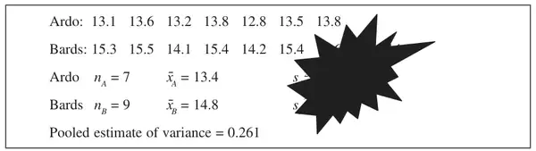
(a) State one other assumption that must be made in order to apply this test and show that this assumption is reasonable by testing it at a 10% level of significance. State your hypotheses clearly. (7)
(b) Stating your hypotheses clearly, test, using a significance level of 5%, whether or not there is a difference between the mean marks of the two groups of students. (7)
Mark scheme (a)
Scheme
Marks
The variance of the two group’s marks must be the same.
4. A random sample of 8 people were given a new drug designed to help people sleep.
In a two-week period the drug was given for one week and a placebo (a tablet that contained no drug) was given for one week.
In the first week 4 people, selected at random, were given the drug and the other 4 people were given the placebo. Those who were given the drug in the first week were given the placebo in the second week. Those who were given the placebo in the first week were given the drug in the second week.
The mean numbers of hours of sleep per night for each of the people are shown in the table.
Person
\(A\)
\(B\)
\(C\)
\(D\)
\(E\)
\(F\)
\(G\)
\(H\)
Hours of sleep with drug
10.8
7.2
8.7
6.8
9.4
10.9
11.1
7.6
Hours of sleep with placebo
10.0
6.5
9.0
5.6
8.7
8.0
9.8
6.8
(a) State one assumption that needs to be made in order to carry out a paired \(t\)-test. (1)
(b) Stating your hypotheses clearly, test, at the 1% level of significance, whether or not the drug increases the mean number of hours of sleep per night by more than 10 minutes. State the critical value for this test. (8)
Mark scheme (a)
Scheme
Marks
The differences in the mean number of hours sleep are normally distributed
B1
(1)
Notes
B1 for a comment that mentions “differences” and “normal” distribution
Mark scheme (b)
Scheme
Marks
Differences are 0.8, 0.7, −0.3, 1.2, 0.7, 2.9, 1.3, 0.8
M1
\(\bar{d} = \frac{8.1}{8} = 1.0125\)
M1
\(s_d = \sqrt{\frac{13.89 - 8 \times 1.0125^2}{7}} = 0.901\ldots\) both \(\bar{d}\) and s
There is insufficient evidence to suggest the drugincreases the mean number of hours slept by more than 10 minutes.
A1ft
(8)
(9 marks)
Notes
1st M1 for attempting the \(d\)s
2nd M1 for attempting \(\bar{d}\)
1st M1 for \(s_d\) or \({s_d}^2\)
1st B1 for both hypotheses correct in terms of \(\mu\) or \(\mu_d\). (allow a defined symbol) Do not allow 10 instead of 1/6 (awrt 0.167) unless working in minutes throughout
3rd M1 for attempting the correct test statistic \(\dfrac{\bar{d} - \frac{1}{6}}{s_d/\sqrt{8}}\) or \(p = \text{awrt } 0.016\) or \(\dfrac{c - \frac{1}{6}}{0.901/\sqrt{8}} = t\) value
2nd A1 awrt 2.65 /2.655 or awrt 1.12 or awrt 0.016
2nd B1 2.998 or 0.0164
3rd A1ft for a correct comment in context based on their test statistic and their cv. Do not allow contradictions.
(Corrected from the printed mark scheme: the critical value is printed as 2.988 in the CR working and in the 2nd B1 note; \(t_7(1\%) = 2.998\).)
There is evidence to reject \(\mathrm{H}_0\). Malcolm’s belief is supported or there is evidence that the amount of oil placed in bottles is less than 100ml
A1ft
(5)
Notes
B1 both hypotheses
M1 either \(\dfrac{|92.875 - 100|}{8.3055/\sqrt{8}}\) or \(p = 0.0228\) or \(\dfrac{c - 100}{8.3055/\sqrt{8}} = -(\text{a } t \text{ value})\)
A1 awrt 2.43 or awrt 94.4 or awrt 0.0228
B1 \(\pm 1.895\) or \(0.0228 \lt 0.05\) (must have correct comparison for hypotheses) A1ft Do Not allow contradictions
(Corrected from the printed mark scheme: the conclusion printed “100mm” for 100 ml.)
7. A farmer monitored the amount of lead in soil in a field next to a factory. He took 100 samples of soil, randomly selected from different parts of the field, and found the mean weight of lead to be 67 mg/kg with standard deviation 25 mg/kg.
After the factory closed, the farmer took 150 samples of soil, randomly selected from different parts of the field, and found the mean weight of lead to be 60 mg/kg with standard deviation 10 mg/kg.
(a) Test at the 5% level of significance whether or not the mean weight of lead in the soil decreased after the factory closed. State your hypotheses clearly. (7)
(b) Explain the significance of the Central Limit Theorem to the test in part (a). (1)
(c) State an assumption you have made to carry out this test. (1)
One tailed critical value \(z = 1.6449\) (or prob of awrt 0.004 (<0.05)) [Condone 0.996 if compared correctly with 0.95 for the B1]
B1
[2.6616 > 1.6449 so] significant evidence to reject \(\mathrm{H_0}\)
dM1
There is evidence that the amount of lead present in the soil has decreased.
A1ft
(7)
Notes
1st B1 for both hypotheses in terms of \(\mu\) not words. Accept \(\mu_1, \mu_2\) etc if there is some indication of which is which e.g \(X \sim \mathrm{N}(67, 25^2)\) implies \(X\) is “before”.
1st M1 for attempt at s.e. - condone one number wrong or mis-matched variances i.e. \(\sqrt{\frac{p}{q} + \frac{r}{s}}\) (3 of \(p, q, r\) & \(s\) correct) or \(\sqrt{\frac{10^2}{100} + \frac{25^2}{150}}\)
2nd dM1 Dep on 1st M1 for using their s.e. in correct formula for test statistic. Num of \(\pm(67 - 60)\) or for correct expression for CR
3rd dM1 dep. on 2nd M1 for a correct statement based on their normal cv (\(|\text{cv}| \gt 1.5\)) and their test statistic
2nd A1ft for correct comment in context. Must mention “lead” or “soil” and “factory”. Allow ft If hypotheses are the wrong way round score A0 If hypotheses are not for a difference between 2 means award A0
Mark scheme (b)
Scheme
Marks
CLT enables you to assume that means are normally distributed
B1
(1)
Notes
B1 must mention mean and normal. In words or symbols e.g. \(\bar{X} \sim \mathrm{N}(\ldots\)
Mark scheme (c)
Scheme
Marks
Have assumed \(s^2 = \sigma^2\) or variance of sample = variance of population
6. A machine fills bottles with water. The amount of water in each bottle is normally distributed. To check the machine is working properly, a random sample of 12 bottles is selected and the amount of water, in ml, in each bottle is recorded. Unbiased estimates for the mean and variance are
\[\hat{\mu} = 502 \qquad s^2 = 5.6\]
Stating your hypotheses clearly, test at the 1% level of significance
(a) whether or not the mean amount of water in a bottle is more than 500 ml, (5)
(b) whether or not the standard deviation of the amount of water in a bottle is less than 3 ml. (5)
5. Students studying for their Mathematics GCSE are assessed by two examination papers. A teacher believes that on average the score on paper I is more than 1 mark higher than the score on paper II. To test this belief the scores of 8 randomly selected students are recorded. The results are given in the table below.
Student
\(A\)
\(B\)
\(C\)
\(D\)
\(E\)
\(F\)
\(G\)
\(H\)
Score on paper I
57
63
68
81
43
65
52
31
Score on paper II
53
62
61
78
44
64
43
29
Assuming that the scores are normally distributed and stating your hypotheses clearly, test at the 5% level of significance whether or not there is evidence to support the teacher’s belief. (8)
There is evidence to support the teacher’s belief or the score on paper I is more than one mark higher than on paper II
A1 ft
(8)
(8 marks)
Notes
1st M1 for attempting differences
2nd M1 for attempting \(\bar{d}\)
3rd M1 for attempting \(s_d\) or \({s_d}^2\), correct expression with their \(\sum d^2\) and \(\bar{d}\) or correct calculation (to 2 sf or better)
4th M1 for use of \(\dfrac{\bar{d} - 1}{s/\sqrt{8}}\), ft their values.
1st A1 awrt 1.91
2nd B1 for 1.895
2nd A1 contextual conclusion ft their values.
SC if they use a 2 sample test they may get the first B1 for \(\mathrm{H}_0 : \mu_\mathrm{I} - \mu_\mathrm{II} = 1\) and \(\mathrm{H}_1 : \mu_\mathrm{I} - \mu_\mathrm{II} \gt 1\)
4. A company carries out an investigation into the strengths of rods from two different suppliers, Ardo and Bards. Independent random samples of rods were taken from each supplier and the force, \(x\) kN, needed to break each rod was recorded. The company wrote the results on a piece of paper but unfortunately spilt ink on it so some of the results can not be seen. The paper with the results on is shown below.
(a)
(i) Use the data from Ardo to calculate an unbiased estimate, \(s_A^2\), of the variance.
(ii) Hence find an unbiased estimate, \(s_B^2\), of the variance for the sample of 9 values from Bards. (4)
(b) Stating your hypotheses clearly, test at the 10% level of significance whether or not there is a difference in variability of strength between the rods from Ardo and the rods from Bards. (You may assume the two samples come from independent normal distributions.) (5)
(c) Use a 5% level of significance to test whether the mean strength of rods from Bards is more than 0.9 kN greater than the mean strength of rods from Ardo. (6)
Since 1.94… is in the critical region we reject \(\mathrm{H}_0\) and conclude that the mean strength of rods from Bards is more than 0.9 kN than that from Ardo.
A1 ft
(6)
(15 marks)
Notes
B1 must use \(\mu\). If not use \(A\) and \(B\) it must be clear which is which
M1 for attempt at correct test statistic – matching their hypotheses
1st A1 correct test statistic for their hypotheses
6. The carbon content, measured in suitable units, of steel is normally distributed. Two independent random samples of steel were taken from a refining plant at different times and their carbon content recorded. The results are given below.
Sample \(A\): 1.5 0.9 1.3 1.2
Sample \(B\): 0.4 0.6 0.8 0.3 0.5 0.4
(a) Stating your hypotheses clearly, carry out a suitable test, at the 10% level of significance, to show that both samples can be assumed to have come from populations with a common variance \(\sigma^2\). (7)
(b) Showing your working clearly, find the 99% confidence interval for \(\sigma^2\) based on both samples. (6)
6. Fruit-n-Veg4U Market Gardens grow tomatoes. They want to improve their yield of tomatoes by at least 1 kg per plant by buying a new variety. The variance of the yield of the old variety of plant is 0.5 kg2 and the variance of the yield for the new variety of plant is 0.75 kg2. A random sample of 60 plants of the old variety has a mean yield of 5.5 kg. A random sample of 70 of the new variety has a mean yield of 7 kg.
(a) Stating your hypotheses clearly test, at the 5% level of significance, whether or not there is evidence that the mean yield of the new variety is more than 1 kg greater than the mean yield of the old variety. (9)
(b) Explain the relevance of the Central Limit Theorem to the test in part (a). (2)
[\(3.62 \gt 1.6449\)] so sufficient evidence to reject \(\mathrm{H}_0\)
dM1
Evidence that the mean yield of new variety is more than 1 kg greater than the old variety.
A1
(9)
Notes
1st & 2nd B1 for hypotheses. Accept \(\mu_1, \mu_2\) or \(\mu_A, \mu_B\) etc if there is some indication of which is which e.g. \(A \sim \mathrm{N}(\mu_A, 0.5)\)
1st M1 for an attempt at se. Condone switching 0.5 and 0.75 \(\sqrt{\dfrac{0.5 \text{ or } 0.75}{60} + \dfrac{0.75 \text{ or } 0.5}{70}}\)
1st A1 for a correct expression for denominator of test statistic or 0.138… or \(\sqrt{0.0190\ldots}\)
2nd A1 for a correct numerator of test statistic (must have the \(-1\))
3rd A1 for awrt 3.62 [Allow – 3.62 from numerator of 5.5 – 7 − − 1 and compatible \(\mathrm{H}_1\)]
3rd B1 for \(\pm\) 1.6449 seen or probability of 0.0002 (tables) or 0.000145…(calc) [allow 0.0001]
2nd dM1 dep. on 1st M1 for a correct statement based on their normal cv and their test statistic
2nd A1 for correct comment in context. Must mention “yield” and “varieties” or “old” and “new” and “1” If second B mark is B0 award A0 here
ALT Pooled estimate: If they calculate \(s_p = \sqrt{0.41845\ldots} = 0.64688\ldots\) allow 1st M1, 1st A1 for expression (or awrt 0.114) and 2nd A1 if numerator correct but A0 for test statistic (4.39)
Mark scheme (b)
Scheme
Marks
Mean yield is normally distributed
B1
Sample size is large. Must state or imply that in this case sample size is large
B1
(2)
(11 marks)
Notes
1st B1 for mention of mean (yield) and normal (distribution)
2nd B1 for mention of sample (size) being large in this case
3. An archaeologist is studying the compression strength of bricks at some ancient European sites. He took random samples from two sites \(A\) and \(B\) and recorded the compression strength of these bricks in appropriate units. The results are summarised below.
Site
Sample size (\(n\))
Sample mean (\(\bar{x}\))
Standard deviation (\(s\))
\(A\)
7
8.43
4.24
\(B\)
13
14.31
4.37
It can be assumed that the compression strength of bricks is normally distributed.
(a) Test, at the 2% level of significance, whether or not there is evidence of a difference in the variances of compression strength of the bricks between these two sites. State your hypotheses clearly. (5)
Site \(A\) is older than site \(B\) and the archaeologist claims that the mean compression strength of the bricks was greater at the younger site.
(b) Stating your hypotheses clearly and using a 1% level of significance, test the archaeologist’s claim. (6)
(c) Explain briefly the importance of the test in part (a) to the test in part (b). (1)
sig, there is evidence to support archaeologist’s claim or there is evidence that bricks for site \(B\) have higher mean compression strength than those from site \(A\).
A1ft
(6)
Notes
B1 if \(A\) and \(B\) not used it must be clear which is \(A\) and which is \(B\) 1stM1 for attempt to calculate \(s_p\) or \(s_p^{\,2}\) 2ndM1 for attempt correct test statistic 2ndA1 ft need archaeologist’s or compression
Mark scheme (c)
Scheme
Marks
The test in (b) requires \(\sigma_A^2 = \sigma_B^2\) and the test in part (a) shows that this is a reasonable assumption. (o.e.)
B1
(1)
(12 marks)
Notes
Need to refer to ‘allows us to assume variances the same’ and this is needed in for test. oe
2. Every 6 months some engineers are tested to see if their times, in minutes, to assemble a particular component have changed. The times taken to assemble the component are normally distributed. A random sample of 8 engineers was chosen and their times to assemble the component were recorded in January and in July. The data are given in the table below.
Engineer
\(A\)
\(B\)
\(C\)
\(D\)
\(E\)
\(F\)
\(G\)
\(H\)
January
17
19
22
26
15
28
18
21
July
19
18
25
24
17
25
16
19
(a) Calculate a 95% confidence interval for the mean difference in times. (7)
(b) Use your confidence interval to state, giving a reason, whether or not there is evidence of a change in the mean time to assemble a component. State your hypotheses clearly. (3)
1stM1 for attempting differences 2ndM1 for attempting \(\bar{d}\) 3rdM1 for attempting \(s_d^{\,2}\), correct expression with their \(\sum d^2\) and \(\bar{d}\) or correct calculation (to 2 sf or better) 4thM1 for use of a correct CI formula, using a value for \(t\) and ft their values. 1stA1 for lower limit of -1.57 or -2.32 2ndA1 for corresponding upper limit
S.C. Allow A1A1 for (0, 2.32)
(corrected from the printed mark scheme: the first line is printed as “d = Jan - June”; the second set of times is July) CHECK
Not sig, no evidence of a change in mean time to assemble component
A1ft
(3)
(10 marks)
Notes
B1 for both hypotheses using \(\mu_D\) M1 for a comment about 0 being in (or out) of their interval A1 contextual conclusion – must include assemble components
S.C. If they have used difference in means test in part (a) to get the confidence interval then award the B1 for \(\mathrm{H}_0 : \mu_x - \mu_y = 0 \quad \mathrm{H}_1 : \mu_x - \mu_y \neq 0\) or the correct hypotheses.
1. George owns a garage and he records the mileage of cars, \(x\) thousands of miles, between services. The results from a random sample of 10 cars are summarised below.
\[\sum x = 113.4 \qquad \sum x^2 = 1414.08\]
The mileage of cars between services is normally distributed and George believes that the standard deviation is 2.4 thousand miles.
Stating your hypotheses clearly, test, at the 5% level of significance, whether or not these data support George’s belief. (7)
Significant result, there is evidence of a change in standard deviation or the data do not support George’s belief
A1cso
(7)
(7 marks)
Notes
1stB1 Both hypotheses, must use \(\sigma\). Allow \(\mathrm{H}_0 : \sigma = 2.4 \quad \mathrm{H}_1 : \sigma \neq 2.4\) 1stM1 correct method used 1stA1 awrt 14.2 2ndM1 \(\chi^2 = \dfrac{9 \times \text{"their }s^2\text{"}}{2.4^2}\) 2ndA1 awrt 22.2 2ndB1 for critical value, this should be compatible with their alternative hypothesis (16.919 for one tail test) 3rdA1ft fully correct solution only
5. Boxes of chocolates manufactured by Philippe have a mean weight of \(\mu\) grams and a standard deviation of \(\sigma\) grams. A random sample of 25 of these boxes are weighed. Using this sample, the unbiased estimate of \(\mu\) is 455 and the unbiased estimate of \(\sigma^2\) is 55.
(a) Test, at the 5% level of significance, whether or not \(\sigma\) is greater than 6. State your hypotheses clearly. (6)
(b) Test, at the 5% level of significance, whether or not \(\mu\) is more than 450. (6)
(c) State an assumption you have made in order to carry out the above tests. (1)
A1ft any statement – no conflicting A1ft contextual statement must include “weight of chocolate” and is “greater than 450” (corrected from the printed mark scheme: printed as “greater than 50”) CHECK
5. Mr Alan and Ms Burns are two Mathematics teachers teaching mixed ability groups of students in a large college. At the end of the college year all students took the same examination. A random sample of 29 of Mr Alan’s students and a random sample of 26 of Ms Burns’ students are chosen. The results are summarised in the table below.
Sample Size, \(n\)
Mean, \(\bar{x}\)
Standard Deviation, \(s\)
Mr Alan
29
80
10
Ms Burns
26
74
15
(a) Stating your hypotheses clearly, test, at the 10% level of significance whether there is evidence that there is a difference in the mean scores of their students. (6)
Ms Burns thinks the comparison was unfair as the examination was set by Mr Alan. She looks up a different set of examination results for these students and, although Mr Alan’s sample has a higher mean, she calculates the test statistic for this new set of results to be 1.6
However, Mr Alan now claims that the mean marks of his students are higher than the mean marks of Ms Burns’ students.
(b) Test Mr Alan’s claim, stating the hypotheses and critical values you would use. Use a 10% level of significance. (3)
There is evidence of a difference in the (mean) scores of their students.
A1
(6)
Notes
1st M1 for attempt at s.e. (condone one number wrong) and for using their s.e. in correct formula for test statistic.
1st A1 for correct expression for se
2nd dM1 dep. on 1st M1 for a correct statement based on their normal cv and their test statistic
3rd A1 for correct comment in context. Must mention “scores” and “students / groups/classes” Award A0 for a one-tailed comment.
Mark scheme (b)
Scheme
Marks
(For \(z = 1.6\), test above not significant so no evidence of a difference.) For Mr A’s claim, \(\mathrm{H}_0 : \mu_A = \mu_B\), \(\mathrm{H}_1 : \mu_A \gt \mu_B\), and critical value is \(z = 1.2816\)
3. The sample variance of the lengths of a random sample of 9 paving slabs sold by a builders’ merchant is 36 mm2. The sample variance of the lengths of a random sample of 11 paving slabs sold by a second builders’ merchant is 225 mm2. Test at the 10% significance level whether or not there is evidence that the lengths of paving slabs sold by these builders’ merchants differ in variability. State your hypotheses clearly.
(You may assume the lengths of paving slabs are normally distributed.) (5)
Since 6.25 is in the critical region we can assume that the lengths of paving slabs sold by the builders merchant differ in variability.
A1ft
(5)
(5 marks)
Notes
B1 both correct. Must use \(\sigma\). May use different notation to \(A\) and \(B\) M1 \(\dfrac{225}{36}\) or \(\dfrac{36}{225}\) allow \(\dfrac{15}{6}\) or \(\dfrac{6}{15}\) A1 either 6.25 or 0.16 B1 CR must match their method A1 context must include “lengths of slabs”
2. A biologist investigating the shell size of turtles takes random samples of adult female and adult male turtles and records the length, \(x\) cm, of the shell. The results are summarised below.
Number in sample
Sample mean \(\bar{x}\)
\(\sum x^2\)
Female
6
19.6
2308.01
Male
12
13.7
2262.57
You may assume that the samples come from independent normal distributions with the same variance.
The biologist claims that the mean shell length of adult female turtles is 5 cm longer than the mean shell length of adult male turtles.
(a) Test the biologist’s claim at the 5% level of significance. (10)
(b) Given that the true values for the variance of the population of adult male turtles and adult female turtles are both 0.9 cm2,
(i) show that when samples of size 6 and 12 are used with a 5% level of significance, the biologist’s claim will be accepted if \(4.07 \lt \bar{X}_F - \bar{X}_M \lt 5.93\) where \(\bar{X}_F\) and \(\bar{X}_M\) are the mean shell lengths of females and males respectively.
(ii) Hence find the probability of a type II error for this test if in fact the true mean shell length of adult female turtles is 6 cm more than the mean shell length of adult male turtles. (6)
Since 1.971 is not in the critical region we accept \(\mathrm{H}_0\) and conclude that the mean shell length of female turtles does exceed the shell length of male turtles by 5cm.(or Biologists claim is correct)
A1 ft
(10)
Notes
B1 – awrt 0.61 B1 – awrt 0.935 Both may be implied by correct \(t\) value or \(S_p\) B1 allow rearrangements eg \(\mu_F - \mu_M = 5\). If \(M\) and \(F\) not used then they must make clear what each letter is. B1 CV (if using one tail test allow 1.746) M1 \(\dfrac{5 \times \text{their }0.61 + 11 \times \text{their }0.93545\ldots}{16}\) A1 awrt 0.834 M1 \(\pm\left(\dfrac{19.6 - 13.7 - 5}{\sqrt{p\left(\frac{1}{6} + \frac{1}{12}\right)}}\right)\) where \(p\) is either their 0.61 or 0.94 or their \(S_p^2\) (awrt 0.834) (Allow 13.7 - 19.6 - 5) A1 ft their \(S_p^2\) A1 awrt 1.97
1. A medical student is investigating whether there is a difference in a person’s blood pressure when sitting down and after standing up. She takes a random sample of 12 people and measures their blood pressure, in mmHg, when sitting down and after standing up.
The results are shown below.
Person
\(A\)
\(B\)
\(C\)
\(D\)
\(E\)
\(F\)
\(G\)
\(H\)
\(I\)
\(J\)
\(K\)
\(L\)
Sitting down
135
146
138
146
141
158
136
135
146
161
119
151
Standing up
131
147
132
140
138
160
127
136
142
154
130
144
The student decides to carry out a paired \(t\)-test to investigate whether, on average, the blood pressure of a person when sitting down is more than their blood pressure after standing up.
(a) State clearly the hypotheses that should be used and any necessary assumption that needs to be made. (2)
(b) Carry out the test at the 1% level of significance. (7)
Mark scheme (a)
Scheme
Marks
\(\mathrm{H}_0 : \mu_d = 0,\quad \mathrm{H}_1 : \mu_d \gt 0\) (or \(\mathrm{H}_1 : \mu_d \lt 0\)) where \(\mu_d\) is the (population) mean difference :- BP sitting down – BP standing. (BP standing – BP sitting down)
B1
Assume the differences are normally distributed
B1
(2)
Notes
B1 both hypotheses. B1 must be differences
Mark scheme (b)
Scheme
Marks
\(d\): 4, −1, 6, 6, 3, −2, 9, −1, 4, 7, −11, 7
M1
\((\Sigma d = 31,\ \Sigma d^2 = 419)\quad \bar{d} = \pm 2.5833;\ \mathrm{sd} = 5.55073.\ (\text{ or Var} = 30.8106)\)
A1; A1
\(t = \dfrac{\pm 2.5833\sqrt{12}}{5.55073} = \pm 1.612\ldots\) Formula and substitution, 1.61
M1, A1
Critical value \(t_{11}(1\%) = 2.718\) (1 tail)
B1
Not significant. Insufficient evidence to support that the blood pressure of a person sitting down is more than the blood pressure of a person after standing up.
A1 ft
(7)
(9 marks)
Notes
M1 at least 2 correct or may be implied by correct \(\Sigma d\) or \(\Sigma d^2\) or \(\bar{d}\) or sd or var or implied by correct \(t\) value A1 correct \(\bar{d}\) awrt \(\pm 2.58\)- may be implied by correct \(t\) value A1 correct sd awrt 5.55 or var awrt 30.8 - may be implied by correct \(t\) value M1 \(\dfrac{\pm\text{their }\bar{d}\sqrt{12}}{\text{their sd}}\) A1 awrt 1.61 B1 CV A1ft follow through their \(t\) value – need context of blood pressure and sitting and standing
7. A machine produces components whose lengths are normally distributed with mean 102.3 mm and standard deviation 2.8 mm. After the machine had been serviced, a random sample of 20 components were tested to see if the mean and standard deviation had changed. The lengths, \(x\) mm, of each of these 20 components are summarised as
\[\sum x = 2072 \qquad \sum x^2 = 214\,856\]
(a) Stating your hypotheses clearly, test, at the 5% level of significance, whether or not there is evidence of a change in standard deviation. (7)
(b) Stating your hypotheses clearly, test, at the 5% level of significance, whether or not the mean length of the components has changed from the original value of 102.3 mm using
(i) a normal distribution,
(ii) a \(t\) distribution. (9)
(c) Comment on the mean length of components produced after the service in the light of the tests from part (a) and part (b). Give a reason for your answer. (2)
Critical value is \(z = 1.96\) or awrt \(0.019 \lt 0.025\)
B1
So a significant result, there is evidence of a change in mean length
A1ft
(ii) \(t = \dfrac{\frac{2072}{20} - 102.3}{\sqrt{\frac{10.357\ldots}{20}}} = 1.8064\ldots\) awrt 1.81
M1A1
Critical value of \(t_{19} = 2.093\)
B1
Not significant, there is insufficient evidence of a change in mean length
A1
(9)
Notes
1st and 2ndM1 for use of correct test statistics
Mark scheme (c)
Scheme
Marks
(a) suggests that \(\sigma\) is unchanged so can use \(\sigma = 2.8\) so normal test can be used
B1ft
So using (i) conclude that there is evidence of an increase in mean length
B1ft
(2)
(18 marks)
Notes
1stB1 for reason for selecting (i) or (ii) based on their conclusion from test in (a). 2ndB1 For a final conclusion about mean lengths based on their (a) and (b) NB if both conclusions are the same it needs to be clear they have chosen (i)
7. Roastie’s Coffee is sold in packets with a stated weight of 250 g. A supermarket manager claims that the mean weight of the packets is less than the stated weight. She weighs a random sample of 90 packets from their stock and finds that their weights have a mean of 248 g and a standard deviation of 5.4 g.
(a) Using a 5% level of significance, test whether or not the manager’s claim is justified. State your hypotheses clearly. (5)
(b) Find the 98% confidence interval for the mean weight of a packet of coffee in the supermarket’s stock. (4)
(c) State, with a reason, the action you would recommend the manager to take over the weight of a packet of Roastie’s Coffee. (2)
Roastie’s Coffee company increase the mean weight of their packets to \(\mu\) g and reduce the standard deviation to 3 g. The manager takes a sample of size \(n\) from these new packets. She uses the sample mean \(\overline{X}\) as an estimator of \(\mu\).
(d) Find the minimum value of \(n\) such that \(\mathrm{P}\left(\left|\overline{X} - \mu\right| \lt 1\right) \geqslant 0.98\) (5)
5. The weights of the contents of breakfast cereal boxes are normally distributed. A manufacturer changes the style of the boxes but claims that the weight of the contents remains the same. A random sample of 6 old style boxes had contents with the following weights (in grams).
512 503 514 506 509 515
The weights, \(y\) grams, of the contents of an independent random sample of 5 new style boxes gave
\[\bar{y} = 504.8 \ \text{ and } \ s_y = 3.420\]
(a) Use a two-tail test to show, at the 10% level of significance, that the variances of the weights of the contents of the old and new style boxes can be assumed to be equal. State your hypotheses clearly. (5)
(b) Showing your working clearly, find a 90% confidence interval for \(\mu_x - \mu_y\), where \(\mu_x\) and \(\mu_y\) are the mean weights of the contents of old and new style boxes respectively. (7)
(c) With reference to your confidence interval comment on the manufacturer’s claim. (2)
\(\dfrac{s_x^{\,2}}{s_y^{\,2}} = 1.895\ldots\) awrt 1.90 and comment : not significant - variances of weights of the two boxes can be assumed equal.
A1
(5)
Notes
1stM1 for use of the correct formula for \(s_x^{\,2}\) with reasonable attempt at \(\sum x^2\) and \(\sum x\) 2ndM1 for use of the correct test statistic. Allow use of 3.42 instead of 3.422. Top must be their variance.
1stM1 for attempting \(\bar{x} - \bar{y}\) can follow through their \(\bar{x}\) 2ndM1 for attempt to find pooled estimate of variance 3rdM1 for use of correct formula for CI allow any \(t\) value and ft their \(\bar{x}\) and \(s_p\)
Mark scheme (c)
Scheme
Marks
Zero is not in CI, there is evidence to reject the manufacturer’s claim Or the weight of the contents of the boxes has changed.
4. A shop manager wants to find out if customers spend more money when music is playing in the shop. The amount of money spent by a customer in the shop is £\(x\). A random sample of 80 customers, who were shopping without music playing, and an independent random sample of 60 customers, who were shopping with music playing, were surveyed. The results of both samples are summarised in the table below.
\(\sum x\)
\(\sum x^2\)
Unbiased estimate of mean
Unbiased estimate of variance
Customers shopping without music
5320
392 000
\(\bar{x}\)
\(s^2\)
Customers shopping with music
4140
312 000
69.0
446.44
(a) Find the values of \(\bar{x}\) and \(s^2\). (5)
(b) Test, at the 5% level of significance, whether or not the mean money spent is greater when music is playing in the shop. State your hypotheses clearly. (8)
3. Manuel is planning to buy a new machine to squeeze oranges in his cafe and he has two models, at the same price, on trial. The manufacturers of machine \(B\) claim that their machine produces more juice from an orange than machine \(A\). To test this claim Manuel takes a random sample of 8 oranges, cuts them in half and puts one half in machine \(A\) and the other half in machine \(B\). The amount of juice, in ml, produced by each machine is given in the table below.
Orange
1
2
3
4
5
6
7
8
Machine \(A\)
60
58
55
53
52
51
54
56
Machine \(B\)
61
60
58
52
55
50
52
58
Stating your hypotheses clearly, test, at the 10% level of significance, whether or not the mean amount of juice produced by machine \(B\) is more than the mean amount produced by machine \(A\). (8)
Not significant. There is insufficient evidence to support the claim of manufacturer \(B\) or machine \(B\) does not produce more juice (than machine \(A\))
A1
(8 marks)
Notes
1stM1 for attempting the \(d\)s 2ndM1 for attempting \(\bar{d}\) 3rdM1 for attempting \(s_d\) or \(s_d^{\,2}\) 4thM1 for attempting the correct test statistic 3rdA1 contextual statement only required. Allow The juice provided by machine \(A\) is the same as by machine \(B\)
NB 2 sample test can score 3/8 M0 M0 M1 \(\dfrac{7 \times 9.27 + 7 \times 16.79}{14}\) B1 for \(\mathrm{H}_0 : \mu_A = \mu_B \quad \mathrm{H}_1 : \mu_A \lt \mu_B\) M0 A0 B1 1.345 A0
7. A large company surveyed its staff to investigate the awareness of company policy. The company employs 6000 full time staff and 4000 part time staff.
(a) Describe how a stratified sample of 200 staff could be taken. (3)
(b) Explain an advantage of using a stratified sample rather than a simple random sample. (1)
A random sample of 80 full time staff and an independent random sample of 80 part time staff were given a test of policy awareness. The results are summarised in the table below.
Mean score (\(\bar{x}\))
Variance of scores (\(s^2\))
Full time staff
52
21
Part time staff
50
19
(c) Stating your hypotheses clearly, test, at the 1% level of significance, whether or not the mean policy awareness scores for full time and part time staff are different. (7)
(d) Explain the significance of the Central Limit Theorem to the test in part (c). (2)
(e) State an assumption you have made in carrying out the test in part (c). (1)
After all the staff had completed a training course the 80 full time staff and the 80 part time staff were given another test of policy awareness. The value of the test statistic \(z\) was 2.53
(f) Comment on the awareness of company policy for the full time and part time staff in light of this result. Use a 1% level of significance. (2)
(g) Interpret your answers to part (c) and part (f). (1)
Mark scheme (a)
Scheme
Marks
Label full time staff 1-6000, part time staff 1-4000
M1
Use random numbers to select
M1
Simple random sample of 120 full time staff and 80 part time staff
A1
(3)
Notes
1st M1 for attempt at labelling full-time and part-time staff. One set of correct numbers.
2nd M1 for mentioning use of random numbers
1st A1 for s.r.s. of 120 full-time and 80 part-time
Mark scheme (b)
Scheme
Marks
Enables estimation of statistics / errors for each strata or “reduce variability” or “more representative” or “reflects population structure” NOT “more accurate”
5. A car manufacturer claims that, on a motorway, the mean number of miles per gallon for the Panther car is more than 70. To test this claim a car magazine measures the number of miles per gallon, \(x\), of each of a random sample of 20 Panther cars and obtained the following statistics.
\[\bar{x} = 71.2 \qquad s = 3.4\]
The number of miles per gallon may be assumed to be normally distributed.
(a) Stating your hypotheses clearly and using a 5% level of significance, test the manufacturer’s claim. (5)
The standard deviation of the number of miles per gallon for the Tiger car is 4.
(b) Stating your hypotheses clearly, test, at the 5% level of significance, whether or not there is evidence that the variance of the number of miles per gallon for the Panther car is different from that of the Tiger car. (6)
not significant, insufficient evidence to confirm manufacturer’s claim
A1 ft
(5)
Notes
B1 both hypotheses using \(\mu\) M1 \(\dfrac{71.2 - 70}{3.4/\sqrt{20}}\) A1 awrt 1.58 (corrected from the printed mark scheme: printed as “A1 awrt 1.73”; 1.58 is the test statistic in the scheme above) CHECK A1 correct conclusion ft their \(t\) value and CV
Insufficient evidence to suggest that the variance of the miles per gallon of the panther is different from that of the Tiger.
A1ft
(6)
(11 marks)
Notes
B1 both hypotheses and 16. accept \(\sigma = 4\) and \(\sigma \neq 4\) M1 \(\dfrac{(19) \times 3.4^2}{16}\) allow \(\dfrac{(19) \times 3.4^2}{4}\) A1 awrt 13.7 B1 32.852 B1 8.907 A1 correct contextual comment NB those who use \(\sigma^2 = 4\) throughout can get B0 M1 A0B1 B1 A1
2. As part of an investigation, a random sample of 10 people had their heart rate, in beats per minute, measured whilst standing up and whilst lying down. The results are summarised below.
Person
1
2
3
4
5
6
7
8
9
10
Heart rate lying down
66
70
59
65
72
66
62
69
56
68
Heart rate standing up
75
76
63
67
80
75
65
74
63
75
(a) State one assumption that needs to be made in order to carry out a paired \(t\)-test. (1)
(b) Test, at the 5% level of significance, whether or not there is any evidence that standing up increases people’s mean heart rate by more than 5 beats per minute. State your hypotheses clearly. (8)
Mark scheme (a)
Scheme
Marks
The differences in the mean heart rates are normally distributed.
B1
(1)
Notes
must have “The differences in (mean heart rate) are normally distributed)
Mark scheme (b)
Scheme
Marks
\(D\) = standing up – lying down \(\mathrm{H}_0 : \mu_D = 5 \quad \mathrm{H}_1 : \mu_D \gt 5\)
insignificant. There is no evidence to suggest that heart rate rises by more than 5 beats when standing up.
A1 ft
(8)
(9 marks)
Notes
B1 both correct allow \(\mu_D - 5 \gt 0\) (\(\mu_D = -5 \quad \mathrm{H}_1 : \mu_D \lt -5\)) M1 finding differences M1 finding \(\bar{d}\) M1 \(\sqrt{\dfrac{\sum d^2 - 10 \times (\bar{d})^2}{9}}\) o.e M1 \(\pm\left(\dfrac{6 - 5}{s_d/\sqrt{10}}\right)\) need to see full expression with numbers in A1 awrt \(\pm 1.29\). B1 \(\pm 1.833\) only A1 ft their CV and \(t\). Need context. Heart rate and 5 beats
1. A teacher wishes to test whether playing background music enables students to complete a task more quickly. The same task was completed by 15 students, divided at random into two groups. The first group had background music playing during the task and the second group had no background music playing. The times taken, in minutes, to complete the task are summarised below.
Sample size \(n\)
Standard deviation \(s\)
Mean \(\bar{x}\)
With background music
8
4.1
15.9
Without background music
7
5.2
17.9
You may assume that the times taken to complete the task by the students are two independent random samples from normal distributions.
(a) Stating your hypotheses clearly, test, at the 10% level of significance, whether or not the variances of the times taken to complete the task with and without background music are equal. (5)
(b) Find a 99% confidence interval for the difference in the mean times taken to complete the task with and without background music. (7)
Experiments like this are often performed using the same people in each group.
(c) Explain why this would not be appropriate in this case. (1)
Since 1.61 (0.622) is not in the critical region we accept \(\mathrm{H}_0\) and conclude there is no evidence that the two variances are different
A1ft
(5)
Notes
B1 Allow \(\sigma_1 = \sigma_2\) and \(\sigma_1 \neq \sigma_2\) B1 must match their F M1 for \(\dfrac{s_2^2}{s_1^2}\) or other way up A1 awrt 1.61(0.622)
\(= \pm(9.23,\ -5.233)\), [ or accept: [0, 9.23] or [−9.23, 0] ] awrt 9.23, −5.23
A1A1
(7)
Notes
M1 A1 \(\mathrm{Sp}^2\) may be seen in part a B1 3.012 only M1 for \((17.9 - 15.9) \pm t\text{ value} \times \sqrt{\mathrm{S_p}^2} \times \sqrt{\dfrac{1}{8} + \dfrac{1}{7}}\) A1ft their \(\mathrm{Sp}^2\) A1 awrt 9.23/−9.23 A1 awrt −5.23/5.23
Mark scheme (c)
Scheme
Marks
a person will be quicker at the task second time through/ times not independent/ familiar with the task/groups are not independent
1. A report states that employees spend, on average, 80 minutes every working day on personal use of the Internet. A company takes a random sample of 100 employees and finds their mean personal Internet use is 83 minutes with a standard deviation of 15 minutes. The company’s managing director claims that his employees spend more time on average on personal use of the Internet than the report states.
Test, at the 5% level of significance, the managing director’s claim. State your hypotheses clearly. (7)
Reject \(\mathrm{H}_0\) or significant result or in the critical region
M1
Managing director’s claim is supported.
A1
(7 marks)
Notes
1st B1 for \(\mathrm{H}_0\). They must use \(\mu\) not \(x\), \(p\), \(\lambda\) or \(\bar{x}\) etc
2nd B1 for \(\mathrm{H}_1\) (must be > 80). Same rules about \(\mu\).
1st M1 for attempt at standardising using 83, 80 and \(\dfrac{15}{\sqrt{100}}\). Can accept \(\pm\). May be implied by \(z = \pm 2\)
1st A1 for + 2 only
3rd B1 for \(\pm\)1.6449 seen (or probability of 0.0228 or better)
2nd M1 for a correct statement about “significance” or rejecting \(\mathrm{H}_0\) (or \(\mathrm{H}_1\)) based on their \(z\) value and their 1.6449 (provided it is a recognizable critical value from normal tables) or their probability (< 0.5) and significance level of 0.05. Condone their probability > 0.5 compared with 0.95 for the 2nd M1
2nd A1 for a correct contextualised comment. Must mention “director” and “claim” or “time” and “use of Internet”. No follow through.
2nd M1A1 If no comparison or statement is made but a correct contextualised comment is given the M1 can be implied. If a comparison is made it must be compatible with statement otherwise M0 e.g. comparing 0.0228 with 1.6449 is M0 or comparing probability 0.9772 with 0.05 is M0 comparing -2 with - 1.6449 is OK provided a correct statement accompanies it condone -2 >-1.6449 provided their statement correctly rejects \(\mathrm{H}_0\).
Critical Region They may find a critical region for \(\overline{X}\) : \(\overline{X} \gt 80 + \dfrac{15}{\sqrt{100}} \times 1.6449 =\) awrt 82.5 1st M1 for \(80 + \dfrac{15}{\sqrt{100}} \times (z \text{ value})\) 3rd B1 for 1.645 or better 1st A1 for awrt 82.5 The rest of the marks are as per the scheme.
6. The lengths of a random sample of 120 limpets taken from the upper shore of a beach had a mean of 4.97 cm and a standard deviation of 0.42 cm. The lengths of a second random sample of 150 limpets taken from the lower shore of the same beach had a mean of 5.05 cm and a standard deviation of 0.67 cm.
(a) Test, using a 5% level of significance, whether or not the mean length of limpets from the upper shore is less than the mean length of limpets from the lower shore. State your hypotheses clearly. (8)
(b) State two assumptions you made in carrying out the test in part (a). (2)
Mark scheme (a)
Scheme
Marks
\(\mu_{\mathrm{U}}\) ~ mean length of upper shore limpets, \(\mu_{\mathrm{L}}\) ~ mean length of lower shore limpets \(\mathrm{H}_0 : \mu_{\mathrm{u}} = \mu_{\mathrm{L}}\) \(\mathrm{H}_1 : \mu_{\mathrm{u}} \lt \mu_{\mathrm{L}}\) both
Critical region is \(z \geqslant 1.6449\), or probability = awrt (0.115 or 0.116) \(z = \pm 1.6449\)
B1
(\(1.1975 \lt 1.6449\)) therefore not in critical region / accept \(\mathrm{H}_0\)/not significant (or \(\mathrm{P}(Z \geqslant 1.1975) = 0.1151,\ 0.1151 \gt 0.05\) or z not in critical region )
M1
There is no evidence that the limpets on the upper shore are shorter than the limpets on the lower shore.
A1
(8)
Notes
1st B1 If \(\mu_1, \mu_2\) used then it must be clear which refers to upper shore. Accept sensible choice of letters such as \(u\) and \(l\).
1st M1 Condone minor slips e.g. \(\dfrac{0.67^2}{120}\) or \(\dfrac{0.67}{150} + \dfrac{0.42^2}{120}\) etc i.e. swapped \(n\) or one sd and one variance but M0 for \(\sqrt{\dfrac{0.67}{150} + \dfrac{0.42}{120}}\)
1st A1 can be scored for a fully correct expression. May be implied by awrt 1.20
2nd dM1 is dependent upon the 1st M1 but can ft their se value if this mark is scored.
2nd A1 for awrt (\(\pm\)) 1.20
3rd M1 for a correct statement based on their \(z\) value and their cv. No cv is M0A0 If using probability they must compare their \(p\) (<0.5) with 0.05 (o.e) so can allow 0.884< 0.95 to score this 3rd M1 mark. May be implied by their contextual statement and M1A0 is possible.
3rd A1 for a correct comment to accept null hypothesis that mentions length of limpets on the two shores.
Mark scheme (b)
Scheme
Marks
Assume the populations or variables are independent
B1
Standard deviation of sample = standard deviation of population [Mention of Central Limit Theorem does NOT score the mark]
B1
(2)
(10 marks)
Notes
1st B1 for one correct statement. Accept ”samples are independent”
4. A farmer set up a trial to assess whether adding water to dry feed increases the milk yield of his cows. He randomly selected 22 cows. Thirteen of the cows were given dry feed and the other 9 cows were given the feed with water added. The milk yields, in litres per day, were recorded with the following results.
Sample size
Mean
\(s^2\)
Dry feed
13
25.54
2.45
Feed with water added
9
27.94
1.02
You may assume that the milk yield from cows given the dry feed and the milk yield from cows given the feed with water added are from independent normal distributions.
(a) Test, at the 10% level of significance, whether or not the variances of the populations from which the samples are drawn are the same. State your hypotheses clearly. (5)
(b) Calculate a 95% confidence interval for the difference between the two mean milk yields. (7)
(c) Explain the importance of the test in part (a) to the calculation in part (b). (2)
2. An emission-control device is tested to see if it reduces CO2 emissions from cars. The emissions from 6 randomly selected cars are measured with and without the device. The results are as follows.
Car
\(A\)
\(B\)
\(C\)
\(D\)
\(E\)
\(F\)
Emissions without device
151.4
164.3
168.5
148.2
139.4
151.2
Emissions with device
148.9
162.7
166.9
150.1
140.0
146.7
(a) State an assumption that needs to be made in order to carry out a \(t\)-test in this case. (1)
(b) State why a paired \(t\)-test is suitable for use with these data. (1)
(c) Using a 5% level of significance, test whether or not there is evidence that the device reduces CO2 emissions from cars. (8)
(d) Explain, in context, what a type II error would be in this case. (2)
Mark scheme (a)
Scheme
Marks
The differences are normally distributed
B1
(1)
Mark scheme (b)
Scheme
Marks
The data is collected in pairs or small sample size and variance unknown or samples not independent
B1
(1)
Notes
Allow because the same car has been used
Mark scheme (c)
Scheme
Marks
\(d\): 2.5, 1.6, 1.6, −1.9, −0.6, 4.5 at least 2 correct
\(\mathrm{H}_0 : \mu_d = 0,\ \mathrm{H}_1 : \mu_d \gt 0\) (\(\mathrm{H}_1 : \mu_d \lt 0\) if \(d\) −2.5, −1.6, −1.6 etc) both depend on their \(d\)’s
B1
\(t = \dfrac{\pm 1.2833\sqrt{6}}{2.2675} = \pm 1.386\ldots\) formula and substitution, 1.38 – 1.39
M1, A1
Critical value \(t_5(5\%) = 2.015\) (1 tail)
B1
Not significant. Insufficient evidence to support that the device reduces CO2 emissions.
A1 ft
(8)
Notes
awrt \(\pm 1.28\), 2.27
Mark scheme (d)
Scheme
Marks
The idea that the device reduces CO2 emissions has been rejected when in fact it does reduce emissions. OR Concluding that the device does not reduce emissions when in fact it does (if not in context can get B1 only)
1. A company manufactures bolts with a mean diameter of 5 mm. The company wishes to check that the diameter of the bolts has not decreased. A random sample of 10 bolts is taken and the diameters, \(x\) mm, of the bolts are measured. The results are summarised below.
\[\sum x = 49.1 \qquad \sum x^2 = 241.2\]
Using a 1% level of significance, test whether or not the mean diameter of the bolts is less than 5 mm.
(You may assume that the diameter of the bolts follows a normal distribution.) (8)
Since 2.475 is not in the critical region there is insufficient evidence to reject \(\mathrm{H}_0\) and conclude that the mean diameter of the bolts is not less than (not equal to) 5 mm.
7. An engineering firm buys steel rods. The steel rods from its present supplier are known to have a mean tensile strength of 230 N/mm2.
A new supplier of steel rods offers to supply rods at a cheaper price than the present supplier. A random sample of ten rods from this new supplier gave tensile strengths, \(x\) N/mm2, which are summarised below.
Sample size
\(\Sigma x\)
\(\Sigma x^2\)
10
2283
524 079
(a) Stating your hypotheses clearly, and using a 5% level of significance, test whether or not the rods from the new supplier have a tensile strength lower than the present supplier. (You may assume that the tensile strength is normally distributed). (7)
(b) In the light of your conclusion to part (a) write down what you would recommend the engineering firm to do. (1)
7. A sociologist is studying how much junk food teenagers eat. A random sample of 100 female teenagers and an independent random sample of 200 male teenagers were asked to estimate what their weekly expenditure on junk food was. The results are summarised below.
\(n\)
mean
s.d.
Female teenagers
100
£5.48
£3.62
Male teenagers
200
£6.86
£4.51
(a) Using a 5% significance level, test whether or not there is a difference in the mean amounts spent on junk food by male teenagers and female teenagers. State your hypotheses clearly. (7)
(b) Explain briefly the importance of the central limit theorem in this problem. (1)
2 tail 5% critical value (\(\pm\)) 1.96 (or probability awrt 0.0021~0.0022)
B1
Significant result or reject the null hypothesis (o.e.)
M1
There is evidence of a difference in the (mean) amount spent on junk food by male and female teenagers
A1ft
(7)
Notes
1st M1 for an attempt at \(\dfrac{a - b}{\sqrt{\dfrac{c}{100 \text{ or } 200} + \dfrac{d}{100 \text{ or } 200}}}\) with 3 of \(a\), \(b\), \(c\) or \(d\) correct 1st A1 for a fully correct expression
2nd B1 for \(\pm\) 1.96 but only if their \(\mathrm{H}_1\) is two-tail (it may be in words so B0B1 is OK) If \(\mathrm{H}_1\) is one-tail this is automatically B0 too.
2nd M1 for a correct statement based on comparison of their \(z\) with their cv. May be implied 3rd A1 for a correct conclusion in context based on their \(z\) and 1.96. Must mention junk food or money and male vs female.
Mark scheme (b)
Scheme
Marks
CLT enables us to assume \(\bar{F}\) and \(\bar{M}\) are normally distributed
B1
(1)
(8 marks)
Notes
B1 for \(\bar{F}\) or \(\bar{M}\) mentioned. Allow “mean (amount spent on junk food) is normally distributed” Read the whole statement e.g. “original distribution is normal so mean is…” scores B0
3. The weights, in grams, of mice are normally distributed. A biologist takes a random sample of 10 mice. She weighs each mouse and records its weight.
The ten mice are then fed on a special diet. They are weighed again after two weeks.
Their weights in grams are as follows:
Mouse
A
B
C
D
E
F
G
H
I
J
Weight before diet
50.0
48.3
47.5
54.0
38.9
42.7
50.1
46.8
40.3
41.2
Weight after diet
52.1
47.6
50.1
52.3
42.2
44.3
51.8
48.0
41.9
43.6
Stating your hypotheses clearly, and using a 1% level of significance, test whether or not the diet causes an increase in the mean weight of the mice. (8)
2. A large number of students are split into two groups \(A\) and \(B\). The students sit the same test but under different conditions. Group \(A\) has music playing in the room during the test, and group \(B\) has no music playing during the test. Small samples are then taken from each group and their marks recorded. The marks are normally distributed.
The marks are as follows:
Sample from Group \(A\)
42
40
35
37
34
43
42
44
49
Sample from Group \(B\)
40
44
38
47
38
37
33
(a) Stating your hypotheses clearly, and using a 10% level of significance, test whether or not there is evidence of a difference between the variances of the marks of the two groups. (8)
(b) State clearly an assumption you have made to enable you to carry out the test in part (a). (1)
(c) Use a two tailed test, with a 5% level of significance, to determine if the playing of music during the test has made any difference in the mean marks of the two groups. State your hypotheses clearly. (7)
(d) Write down what you can conclude about the effect of music on a student’s performance during the test. (1)
\(1.04 \lt 4.15\) do not reject \(\mathrm{H}_0\). The variances are the same.
B1
(8)
Notes
(corrected from the printed mark scheme: the scheme prints the hypotheses with the labels swapped, “\(\mathrm{H}_1 : \sigma_A^2 = \sigma_B^2 \quad \mathrm{H}_0 : \sigma_A^2 \neq \sigma_B^2\)”)
Mark scheme (b)
Scheme
Marks
Assume the samples are selected at random, (independent)
5. In a trial of diet \(A\) a random sample of 80 participants were asked to record their weight loss, \(x\) kg, after their first week of using the diet. The results are summarised by
(a) Find unbiased estimates for the mean and variance of weight lost after the first week of using diet \(A\). (5)
The designers of diet \(A\) believe it can achieve a greater mean weight loss after the first week than a standard diet \(B\). A random sample of 60 people used diet \(B\). After the first week they had achieved a mean weight loss of 4.06 kg, with an unbiased estimate of variance of weight loss of 2.50 kg2.
(b) Test, at the 5% level of significance, whether or not the mean weight loss after the first week using diet \(A\) is greater than that using diet \(B\). State your hypotheses clearly. (7)
(c) Explain the significance of the central limit theorem to the test in part (b). (1)
(d) State an assumption you have made in carrying out the test in part (b). (1)
One tail c.v. is \(z = 1.6449\) (AWRT 1.645 or probability AWRT 0.0307 or 0.0308)
B1
(significant) there is evidence that diet \(A\) is better than diet \(B\) or evidence that (mean) weight lost in first week using diet \(A\) is more than with \(B\)
A1ft
(7)
Notes
1st B1 can be given for \(\mu_1 = \mu_2\), but 2nd B1 must specify which is \(A\) or \(B\).
1st M1 for the denominator, follow through their 1.51. Must have square root can condone \(2.50^2\) but \(\sqrt{\dfrac{1.51^2}{80} + \dfrac{2.50^2}{60}}\) is M0. Allow \(\sqrt{\dfrac{1.51}{79} + \dfrac{2.50}{59}}\) leading to AWRT 1.85 to score M1M1A0 in (b) and can score in (d).
2nd dM1 for attempting the correct test statistic, dependent on denominator mark 1st A1 for AWRT \(\pm\) 1.87, may be implied by a correct probability. 2nd A1ft ft their test statistic vs their cv only if \(\mathrm{H}_1\) is correct and both Ms are scored
Mark scheme (c)
Scheme
Marks
CLT enables you to assume that \(\bar{A}\) and \(\bar{B}\) are normally distributed
B1
(1)
Notes
B1 for stating either \(\bar{A}\) or \(\bar{B}\) (but not \(A\) or \(B\)) are normally distributed
Mark scheme (d)
Scheme
Marks
Assumed \(\sigma_A^{\,2} = s_A^{\,2}\) and \(\sigma_B^{\,2} = s_B^{\,2}\) (either)
B1
(1)
(14 marks)
Notes
B1 for either, can be stated in words in terms of variances or standard deviations.
4. The length \(X\) mm of a spring made by a machine is normally distributed \(\mathrm{N}(\mu, \sigma^2)\). A random sample of 20 springs is selected and their lengths measured in mm. Using this sample the unbiased estimates of \(\mu\) and \(\sigma^2\) are
\[\bar{x} = 100.6, \qquad s^2 = 1.5.\]
Stating your hypotheses clearly test, at the 10% level of significance,
(a) whether or not the variance of the lengths of springs is different from 0.9, (6)
(b) whether or not the mean length of the springs is greater than 100 mm. (6)
3. The lengths, \(x\) mm, of the forewings of a random sample of male and female adult butterflies are measured. The following statistics are obtained from the data.
No. of butterflies
Sample mean \(\bar{x}\)
\(\sum x^2\)
Females
7
50.6
17 956.5
Males
10
53.2
28 335.1
(a) Assuming the lengths of the forewings are normally distributed test, at the 10% level of significance, whether or not the variances of the two distributions are the same. State your hypotheses clearly. (7)
(b) Stating your hypotheses clearly test, at the 5% level of significance, whether the mean length of the forewings of the female butterflies is less than the mean length of the forewings of the male butterflies. (6)
3. The time, in minutes, it takes Robert to complete the puzzle in his morning newspaper each day is normally distributed with mean 18 and standard deviation 3. After taking a holiday, Robert records the times taken to complete a random sample of 15 puzzles and he finds that the mean time is 16.5 minutes. You may assume that the holiday has not changed the standard deviation of times taken to complete the puzzle.
Stating your hypotheses clearly test, at the 5% level of significance, whether or not there has been a reduction in the mean time Robert takes to complete the puzzle. (7)
5% one tail c.v. is \(z = (-)\,1.6449\) or probability (AWRT 0.026) (\(\pm\)) 1.6449
B1
\(-1.94 \lt -1.6449\) or significant or reject \(\mathrm{H}_0\) or in critical region
M1
There is evidence that the (mean) time to complete the puzzles has reduced Or Robert is getting faster (at doing the puzzles)
A1f.t.
(7)
(7 marks)
Notes
1st & 2nd B1 must see \(\mu\) and 18
1st M1 for attempting test statistic, allow \(\pm\). Or attempt at critical value for \(\bar{X}\): \(\mu - z \times \dfrac{3}{\sqrt{15}}\)
1st A1 for AWRT −1.94. Allow use of \(|z| = +1.94\) to score M1A1. Or critical value = AWRT 16.7.
3rd B1 for AWRT 0.026 (i.e. correct probability only) or \(\pm\) 1.6449. (May be seen in cv formula)
2nd M1 for correct comparison or statement relating their test statistic and 1.6449 or their probability and 0.05. Ignore their hypotheses if any or assume they were correct.
2nd A1f.t. for conclusion in context which refers to “speed” or “time”. Depends only on previous M
1. A medical student is investigating two methods of taking a person’s blood pressure. He takes a random sample of 10 people and measures their blood pressure using an arm cuff and a finger monitor. The table below shows the blood pressure for each person, measured by each method.
Person
A
B
C
D
E
F
G
H
I
J
Arm cuff
140
110
138
127
142
112
122
128
132
160
Finger monitor
154
112
156
152
142
104
126
132
144
180
(a) Use a paired \(t\)-test to determine, at the 10% level of significance, whether or not there is a difference in the mean blood pressure measured using the two methods. State your hypotheses clearly. (8)
(b) State an assumption about the underlying distribution of measured blood pressure required for this test. (1)
4. Two machines \(A\) and \(B\) produce the same type of component in a factory. The factory manager wishes to know whether the lengths, \(x\) cm, of the components produced by the two machines have the same mean. The manager took a random sample of components from each machine and the results are summarised in the table below.
Sample size
Mean \(\bar{x}\)
Standard deviation \(s\)
Machine \(A\)
9
4.83
0.721
Machine \(B\)
10
4.85
0.572
The lengths of components produced by the machines can be assumed to follow normal distributions.
(a) Use a two tail test to show, at the 10% significance level, that the variances of the lengths of components produced by each machine can be assumed to be equal. (4)
(b) Showing your working clearly, find a 95% confidence interval for \(\mu_B - \mu_A\), where \(\mu_A\) and \(\mu_B\) are the mean lengths of the populations of components produced by machine \(A\) and machine \(B\) respectively. (7)
There are serious consequences for the production at the factory if the difference in mean lengths of the components produced by the two machines is more than 0.7 cm.
(c) State, giving your reason, whether or not the factory manager should be concerned. (2)
3. As part of an investigation into the effectiveness of solar heating, a pair of houses was identified where the mean weekly fuel consumption was the same. One of the houses was then fitted with solar heating and the other was not. Following the fitting of the solar heating, a random sample of 9 weeks was taken and the table below shows the weekly fuel consumption for each house.
Week
1
2
3
4
5
6
7
8
9
Without solar heating
19
19
18
14
6
7
5
31
43
With solar heating
13
22
11
16
14
1
0
20
38
Units of fuel used per week
(a) Stating your hypotheses clearly, test, at the 5% level of significance, whether or not there is evidence that the solar heating reduces the mean weekly fuel consumption. (8)
(b) State an assumption about weekly fuel consumption that is required to carry out this test. (1)
Mark scheme (a)
Scheme
Marks
(\(D\) = Without Solar heating − with Solar heating) \(\mathrm{H}_0 : \mu_D = 0 \qquad \mathrm{H}_1 : \mu_D \gt 0\)
3. A biologist investigated whether or not the diet of chickens influenced the amount of cholesterol in their eggs. The cholesterol content of 70 eggs selected at random from chickens fed diet \(A\) had a mean value of 198 mg and a standard deviation of 47 mg. A random sample of 90 eggs from chickens fed diet \(B\) had a mean cholesterol content of 201 mg and a standard deviation of 23 mg.
(a) Stating your hypotheses clearly and using a 5% level of significance, test whether or not there is a difference between the mean cholesterol content of eggs laid by chickens fed on these two diets. (7)
(b) State, in the context of this question, an assumption you have made in carrying out the test in part (a). (2)
Mark scheme (a)
Scheme
Marks
\(\mathrm{H}_0 : \mu_A = \mu_B\), \(\mathrm{H}_1 : \mu_A \neq \mu_B\) \(\mu_1, \mu_2\) OK both
Insufficient evidence to reject \(\mathrm{H}_0\), no significant difference between the mean cholesterol content of the two samples. (require correct comparison for ft) context required.
A1ft
(7)
Mark scheme (b)
Scheme
Marks
– require 1 egg from each of 70 chickens of diet \(A\) to ensure independence, similarly for diet \(B\). – no chickens in common between the two samples to ensure independence – not same chickens on diet \(A\) and diet \(B\) because if it were we need to do a paired analysis. Any 1
2. The weights, in grams, of apples are assumed to follow a normal distribution.
The weights of apples sold by a supermarket have variance \(\sigma_s^2\). A random sample of 4 apples from the supermarket had weights
114, 110, 119, 123.
(a) Find a 95% confidence interval for \(\sigma_s^2\). (7)
The weights of apples sold on a market stall have variance \(\sigma_M^2\). A second random sample of 7 apples was taken from the market stall. The sample variance \(s_M^2\) of the apples was 318.8.
(b) Stating your hypotheses clearly test, at the 1% level of significance, whether or not there is evidence that \(\sigma_M^2 \gt \sigma_s^2\). (5)
Mark scheme (a)
Scheme
Marks
\(\left(\bar{x} = \dfrac{466}{4} = 116.5\right) \qquad s_x^2 = \dfrac{54386 - 4\bar{x}^2}{3},\ = 32.\dot{3}\) or \(\dfrac{97}{3}\) or awrt 32.3
The question paper file gives the second weight as 100; the mark scheme’s working (\(\Sigma x = 466\), \(\Sigma x^2 = 54\,386\)) uses 110, so the question is shown here with 110.
Mark scheme (b)
Scheme
Marks
\(\mathrm{H}_0 : \sigma_M^2 = \sigma_s^2 \qquad \mathrm{H}_1 : \sigma_M^2 \gt \sigma_s^2\) both (\(\sigma_M = \sigma_s\), \(\sigma_M \gt \sigma_s\) are OK)
\(9.86 \lt 27.91\), insufficient evidence of an increase in variance … to say \(\sigma_M^2 \gt \sigma_s^2\) is OK. … variance can be assumed to be the same is OK
A1ft
(5)
(12 marks)
Notes
NB \(\dfrac{32.\dot{3}}{318.8} = 0.101\ldots\) only gets M1 A1 if appropriate F value attempted
1. Historical records from a large colony of squirrels show that the weight of squirrels is normally distributed with a mean of 1012 g. Following a change in the diet of squirrels, a biologist is interested in whether or not the mean weight has changed.
A random sample of 14 squirrels is weighed and their weights \(x\), in grams, recorded. The results are summarised as follows:
\[\Sigma x = 13\,700, \qquad \Sigma x^2 = 13\,448\,750.\]
Stating your hypotheses clearly test, at the 5% level of significance, whether or not there has been a change in the mean weight of the squirrels. (7)
7. A psychologist gives a test to students from two different schools, \(A\) and \(B\). A group of 9 students is randomly selected from school \(A\) and given instructions on how to do the test. A group of 7 students is randomly selected from school \(B\) and given the test without the instructions.
The table shows the time taken, to the nearest second, to complete the test by the two groups.
\(A\)
11
12
12
13
14
15
16
17
17
\(B\)
8
10
11
13
13
14
14
Stating your hypotheses clearly,
(a) test at the 10% significance level, whether or not the variance of the times taken to complete the test by students from school \(A\) is the same as the variance of the times taken to complete the test by students from school \(B\). (You may assume that times taken for each school are normally distributed.) (7)
(b) test at the 5% significance level, whether or not the mean time taken to complete the test by students from school \(A\) is greater than the mean time taken to complete the test by students from school \(B\). (7)
(c) Why does the result to part (a) enable you to carry out the test in part (b)? (1)
(d) Give one factor that has not been taken into account in your analysis. (1)
5. Seven pipes of equal length are selected at random. Each pipe is cut in half. One piece of each pipe is coated with protective paint and the other is left uncoated. All of the pieces of pipe are buried to the same depth in various soils for 6 months.
The table gives the percentage area of the pieces of pipe in the various soils that are subject to corrosion.
Soil
A
B
C
D
E
F
G
% Corrosion coated pipe
39
40
43
32
42
33
36
% Corrosion uncoated pipe
41
36
61
48
42
48
45
(a) Stating your hypotheses clearly and using a 5% significance level, carry out a paired \(t\)-test to assess whether or not there is a difference between the mean percentage of corrosion on the coated pipes and the mean percentage of corrosion on the uncoated pipes. (9)
(b)
(i) State an assumption that has been made in order to carry out this test. (1)
(ii) Comment on the validity of this assumption. (1)
(c) State what difference would be made to the conclusion in part (a) if the test had been to determine whether or not the percentage of corrosion on the uncoated pipes was higher than the mean percentage of corrosion on the coated pipes. Justify your answer. (2)
Insufficient evidence to reject \(\mathrm{H}_0\). No evidence of a difference between the mean amount of corrosion on coated and uncoated pipes.
A1
(9)
Mark scheme (b)
Scheme
Marks
(i) Differences are normally distributed
B1
(1)
(ii) Values do not appear to be normally distributed
B1
(1)
Mark scheme (c)
Scheme
Marks
\(t_6(5\%) = 1.943\). There is evidence to reject \(\mathrm{H}_0\).
B1
There is evidence to suggest that there is a greater corrosion on uncoated pipes.
B1
(2)
(13 marks)
Notes
(corrected from the printed mark scheme: the scheme prints “greater corrosion on coated pipes”; with \(d = U - C\) and \(\bar{d} = 8 \gt 0\) the greater corrosion is on the uncoated pipes)
5. Upon entering a school, a random sample of eight girls and an independent random sample of eighty boys were given the same examination in mathematics. The girls and boys were then taught in separate classes. After one year, they were all given another common examination in mathematics.
The means and standard deviations of the boys’ and the girls’ marks are shown in the table.
Examination marks
Upon entry
After 1 year
Mean
Standard deviation
Mean
Standard deviation
Boys
50
12
59
6
Girls
53
12
62
6
You may assume that the test results are normally distributed.
(a) Test, at the 5% level of significance, whether or not the difference between the means of the boys’ and girls’ results was significant when they entered school. (7)
(b) Test, at the 5% level of significance, whether or not the mean mark of the boys is significantly less than the mean mark of the girls in the ‘After 1 year’ examination. (5)
(c) Interpret the results found in part (a) and part (b). (1)
Mark scheme (a)
Scheme
Marks
\(\mu_b\) = mean mark of boys, \(\mu_g\) = mean mark of girls. \(\mathrm{H}_0 : \mu_b = \mu_g\) \(\mathrm{H}_1 : \mu_b \neq \mu_g\) both
4. A farmer set up a trial to assess the effect of two different diets on the increase in the weight of his lambs. He randomly selected 20 lambs. Ten of the lambs were given diet \(A\) and the other 10 lambs were given diet \(B\). The gain in weight, in kg, of each lamb over the period of the trial was recorded.
(a) State why a paired \(t\)-test is not suitable for use with these data. (1)
(b) Suggest an alternative method for selecting the sample which would make the use of a paired \(t\)-test valid. (1)
(c) Suggest two other factors that the farmer might consider when selecting the sample. (2)
The following paired data were collected.
Diet \(A\)
5
6
7
4.6
6.1
5.7
6.2
7.4
5
3
Diet \(B\)
7
7.2
8
6.4
5.1
7.9
8.2
6.2
6.1
5.8
(d) Using a paired \(t\)-test, at the 5% significance level, test whether or not there is evidence of a difference in the weight gained by the lambs using diet \(A\) compared with those using diet \(B\). (8)
(e) State, giving a reason, which diet you would recommend the farmer to use for his lambs. (1)
Since \(2.8357\ldots\) is in the critical region \((t \gt 2.262)\) there is evidence to reject \(\mathrm{H}_0\). The (mean) weight gained by the lambs is different for each diet.
3. A machine is set to fill bags with flour such that the mean weight is 1010 grams.
To check that the machine is working properly, a random sample of 8 bags is selected. The weight of flour, in grams, in each bag is as follows.
1010 1015 1005 1000 998 1008 1012 1007
Carry out a suitable test, at the 5% significance level, to test whether or not the mean weight of flour in the bags is less than 1010 grams. (You may assume that the weight of flour delivered by the machine is normally distributed.) (8)
Since \(-1.53\) is not in the critical region \((t \lt -1.895)\) there is insufficient evidence to reject \(\mathrm{H}_0\) and thus consistent with the mean weight of flour delivered by the machine is 1010 g.
A1ft
(8)
Notes
(corrected from the printed mark scheme: the scheme prints “awrt 33.7” for \(s^2\); the value it shows is \(33.26785\ldots\), so awrt 33.3)
2. The standard deviation of the length of a random sample of 8 fence posts produced by a timber yard was 8 mm. A second timber yard produced a random sample of 13 fence posts with a standard deviation of 14 mm.
(a) Test, at the 10% significance level, whether or not there is evidence that the lengths of fence posts produced by these timber yards differ in variability. State your hypotheses clearly. (5)
(b) State an assumption you have made in order to carry out the test in part (a). (1)
Since 3.0625 is not in the critical region there is insufficient evidence to reject \(\mathrm{H}_0\). There is insufficient evidence of a difference in the variances of the lengths of the fence posts.
A1ft
(5)
Mark scheme (b)
Scheme
Marks
The distribution of the population of lengths of fence posts is normally distributed.