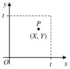
B1: for \(\mathrm{E}(D) = 0\) (May be implied by their other working). May use other letters.
1st M1: for an attempt at \(\bar{X} - Y\) (any expression using \(X_1, X_2, X_3, X_4\) and \(X_5\)). May be seen in attempt to find a probability or \(\mathrm{E}(D)\)
2nd M1: for an attempt to eliminate the “repeats” – condone missing \(\frac{1}{10}\) or errors in “2” and “3”
1st A1: for a correct expression for \(D\) with no “repeats”
3rd dM1: for a correct application of \(\mathrm{Var}(aX - bY)\) dep on 2nd M1 but can ft their expression
2nd A1: for the correct variance (may be implied by a correct answer)
3rd A1: for awrt 0.034
Mark scheme (b)
Scheme
Marks
AO
(27.029, 37.371) since this is the narrower interval or her sample was greater oe
B1
2.2a
(1)
Notes
B1: for choosing the correct interval and giving a suitable reason based on width or sample size. Contradictory or incorrect statements is B0. Do not accept just referring to the standard deviation being smaller without going onto explain the effect on the width of the interval
M1: for an attempt at a correct equation in \(\sigma\). Condone wrong \(n\) and missing \(\times 2\) must have 1.96. Alternatively for an attempt to form two simultaneous equations in \(\bar{x}\) and \(\sigma\), condoning a wrong \(n\). (Condone labelling \(\bar{x}\) as \(\mu\)) Must have 1.96
1st A1: for a correct expression for \(\sigma\). May be implied by awrt 5.9
4. The weights of apples Sam grows are normally distributed with a mean of 131 g and a standard deviation of 6 g
A supermarket will only buy apples with weights in the range 125 g to 137 g
(a) Find the proportion of apples Sam grows that the supermarket will buy. (1)
Some of Sam’s apple trees are treated with the aim of reducing the variability in weight of apples, without significantly affecting the mean weight. The weights of apples are still normally distributed.
A random sample of 25 apples was taken from treated trees and the weight, \(x\) grams, of each apple was recorded. The results are summarised by the following statistics
(b) Use a 5% level of significance to carry out a suitable test to determine whether there is evidence that the variance of the weights of apples from treated trees has decreased. You should clearly state your test statistic, hypotheses and critical value. (6)
(c) Calculate a 95% confidence interval for the mean weight of apples produced by Sam’s trees after treatment. You should clearly state the formula and numerical expression you have used. (3)
(d)
(i) State, giving a reason, whether the aims of the treatment have been met.
(ii) Give an estimate of the proportion of apples the supermarket will buy from Sam’s trees that have been treated. (3)
5% critical value (lower tail) \(\chi^2_{24}(5\%) = 13.848\)
B1
3.4
(Significant result so reject H0) there is evidence that the treatment works oe orvariance of weights is lower oe
A1
2.2b
(6)
Notes
1st B1: for correct hypotheses in terms of \(\sigma\) or \(\sigma^2\) Do not accept in words.
1st M1: for a correct expression for \(s\) or \(s^2\) Implied by \(\dfrac{181}{12}\) or 15.0833…
2nd M1: for a correct expression for ts (ft their 15.0833…) May be implied by awrt 10.1
1st A1: for awrt 10.1 or may see \(\dfrac{181}{18}\)
2nd B1: for the correct cv of 13.848 (accept 13.8 or better or allow 13.85)
2nd A1: for a correct conclusion in context (independent of hypotheses but dep on M2 and their ts < cv where 12 < cv < 15). Incorrect comparison or contradictory statement is A0
M1: for an attempt at a correct formula with 130 or their 3.88… and \(\sqrt{25}\) and \(t \gt 2\)
1st A1ft: for a correct expression using \(t = 2.064\) (or better) can ft their 3.88… = their \(s\)
2nd A1: for awrt (128, 132) provided M1 clearly scored.
Mark scheme (d)
Scheme
Marks
AO
(i) Yes (or treatment worked) since 131 is in CI (and \(\sigma\) reduced)
B1
2.4
(ii) Assume \(\sigma = \) “3.9” (or better) and suitable \(\mu\) e.g. 131
M1
3.5a
Proportion in range (79% ~ 88%)
A1
1.1b
(3)
(13 marks)
Notes
(i) B1: dep on a CI in (c) which includes 131 and concluding variance lower in (b). For stating treatment was successful (o.e. condone e.g. yes) and mentioning 131 (or referred to as the mean) is inside CI. Do not allow reference to critical region for CI.
(ii) M1: for evidence of a suitable \(\sigma\) used (ft their \(s\)) and a value of \(\mu\) from their CI. Must see their values for \(\mu\) and \(\sigma\) to score.
A1: dep on \(\sigma\) = awrt 3.9 and \(\mu = [\text{awrt}\,128,\ \text{awrt}\,132]\) for an answer in the range 0.79 to 0.88 inclusive (decimal or %)
7. Two organisations are each asked to carry out a survey to find out the proportion, \(p\), of the population that would vote for a particular political party.
The first organisation finds that out of \(m\) people, \(X\) would vote for this particular political party.
The second organisation finds that out of \(n\) people, \(Y\) would vote for this particular political party.
An unbiased estimator, \(Q\), of \(p\) is proposed where
\[Q = k\left(\frac{X}{m} + \frac{Y}{n}\right)\]
(a) Show that \(k = \dfrac{1}{2}\) (2)
A second unbiased estimator, \(R\), of \(p\) is proposed where
\[R = \frac{aX}{m} + \frac{bY}{n}\]
(b) Show that \(a + b = 1\) (2)
Given that \(m = 100\) and \(n = 200\) and that \(R\) is a better estimator of \(p\) than \(Q\)
(c) calculate the range of possible values of \(a\) Show your working clearly. (7)
\(2kp = p \qquad\) therefore \(k = \dfrac{1}{2}\)*
A1*
1.1b
(2)
Notes
M1: For selecting the correct models for \(X\) and \(Y\) and subst into \(\mathrm{E}(Q) = k\left(\dfrac{\mathrm{E}(X)}{m} + \dfrac{\mathrm{E}(Y)}{n}\right)\) Both \(mp\) and \(np\) must be seen or used as the expected values for \(X\) and \(Y\). Allow to be implied by \(k\left(\mathrm{E}\left(\dfrac{X}{m}\right) + \mathrm{E}\left(\dfrac{Y}{n}\right)\right) \Rightarrow k(p + p)\) for this mark. Cannot be implied by \(k(p + p)\)
A1*: Cao sets their expression in \(k\) and \(p\) equal to \(p\) before achieving the given answer with no errors.
\(\dfrac{amp}{m} + \dfrac{bnp}{n} = p \quad \therefore a + b = 1\)*
A1*
1.1b
(2)
Notes
M1: Using the model to find \(\mathrm{E}(R)\) in terms of \(a\) and \(b\). Both \(mp\) and \(np\) must be seen or used as the expected values for \(X\) and \(Y\). Must see \(\dfrac{amp}{m} + \dfrac{bnp}{n}\) for this mark. Cannot be implied by \(ap + bp\)
A1*: Cao sets their expression in \(a\), \(b\) and \(p\) equal to \(p\) before achieving the given answer with no errors.
M1: For a correct attempt at \(\mathrm{Var}(Q)\) with at least two of \(m\), \(n\) and 2 being squared on the denominator. May be implied if they cancel by \(m\) or \(n\)
M1: For a correct attempt at \(\mathrm{Var}(R)\) in terms of \(a\) and \(b\) with at least one of \(a\) and \(b\) being squared and at least one of \(m\) and \(n\) being squared. May be implied if they cancel by \(m\) or \(n\) Expression may be in \(a\) only e.g. \(\mathrm{Var}\left(\dfrac{aX}{m} + \dfrac{bY}{n}\right) = \mathrm{Var}\left(\dfrac{aX}{m} + \dfrac{(1-a)Y}{n}\right) = \dfrac{a^2mp(1-p)}{m^2} + \dfrac{(1-a)^2np(1-p)}{n^2}\) Note attempting \(\mathrm{Var}\left(\dfrac{aX}{m} + \dfrac{bY}{n}\right) = \mathrm{Var}\left(\dfrac{aX}{m} + \dfrac{(1-a)Y}{n}\right) = \mathrm{Var}\left(\dfrac{aX}{m} + \dfrac{Y}{n} - \dfrac{aY}{n}\right)\) is M0
M1: using their \(\mathrm{Var}(R) \lt\) their \(\mathrm{Var}(Q)\) condone = instead of < (there must be a term in \(a^2\) in their equation or inequality)
M1: substituting their \(b = 1 - a\) may be scored earlier
M1: forming and solving correctly a 3 term quadratic in \(a\). condone = instead of <
A1: correct values
A1ft: Dep. on all previous M marks and for selecting the right range using their values of \(a\) which must be between 0 and 1
6. A researcher set up a trial to assess the effect that a food supplement has on the increase in weight of Herdwick lambs. The researcher randomly selected 8 sets of twin lambs. One of each set of twins was given the food supplement and the other had no food supplement. The gain in weight, in kg, of each lamb over the period of the trial was recorded.
Set of twin lambs
\(A\)
\(B\)
\(C\)
\(D\)
\(E\)
\(F\)
\(G\)
\(H\)
Weight gain (kg)
With food supplement
4.1
5.3
6.0
3.6
5.9
4.2
7.1
6.4
No food supplement
5.0
4.8
5.2
3.4
5.1
3.9
7.0
6.5
(a) State why a two sample \(t\)-test is not suitable for use with these data. (1)
(b) Suggest 2 other factors about the lambs that the researcher may need to control when selecting the sample. (2)
(c) State one assumption, in context, that needs to be made for a paired \(t\)-test to be valid. (1)
For a pair of twin lambs, the random variable \(W\) represents the weight gain of the lamb given the food supplement minus the weight gain of the lamb not given the food supplement.
(d) Using the data in the table, calculate a 98% confidence interval for the mean of \(W\) Show your working clearly. (5)
The researcher believes that the mean of \(W\) is greater than 200 g
(e) Stating your hypotheses clearly, use your confidence interval to explain whether or not there is evidence to support the researcher’s belief. (3)
Mark scheme (a)
Scheme
Marks
AO
The samples are not independent
B1
3.5b
(1)
Notes
B1: The idea that samples are not independent. Condone other irrelevant comments provided they do not contradict this.
Mark scheme (b)
Scheme
Marks
AO
They should consider the birth weight, gender, or whether or not the lambs are premature. oe
B1 B1
2.4 2.4
(2)
Notes
B1: For one suitable comment on twins being identical relating to selecting the sample. Condone start weight. Do not accept age / diets of the lambs
B1: For a second suitable comment.
Mark scheme (c)
Scheme
Marks
AO
Need the assumption that the underlying distribution of the difference between the weight gains must be normally distributed.
M1: attempting differences (at least 4 correct) implied by awrt 0.304 or 0.551 but not 0.2125
M1: attempt to find \(\bar{w}\) and \(s\) or \(s^2\) for their differences implied by 0.2125 and either awrt 0.304 or 0.551
M1: For using the correct formula their \(\bar{w} \pm t \times \sqrt{\dfrac{\text{their } s^2}{8}}\) where \(|t| \gt 2\) all values need to be substituted in.
A1ft: for their \(\bar{w} \pm\) awrt \(2.998 \times \sqrt{\dfrac{\text{their } s^2}{8}}\) all values need to be substituted in
A1: dependent on all previous method marks (awrt -0.372, awrt 0.797)
SC: If they have carried out a CI for two independent samples allow 3rd M for using their difference of their means and a pooled variance and A1ft using correct formula with awrt 2.624
There is no evidence that \(\mu_w\) is greater than 0.2 oe
A1ft
2.2b
(3)
(12 marks)
Notes
B1: For both hypotheses correct in terms of \(\mu\) or \(\mu_w\) Condone 200
M1: For changing 200 g to 0.2 kg (ignore units for this mark) and comparing to their CI
A1ft: Independent of hypotheses. Drawing a correct inference following through on their CI provided 0.2 is within their confidence interval, with no contradictory statements. Does not need to be in context. Accept “insufficient evidence to support the (researcher’s) belief”.
3. A factory produces bolts. The lengths of the bolts are normally distributed with mean \(\mu\) mm and standard deviation 0.868 mm
A random sample of 15 of these bolts is taken and the mean length is 30.03 mm
(a) Calculate a 90% confidence interval for \(\mu\) (3)
A suitable test, at the 10% level of significance, is carried out using these 15 bolts, to see whether or not there is evidence that the variance of the length of the bolts has increased.
(b) Calculate the critical region for \(S^2\) (3)
The manager of the factory decides that, in future, he will check each month whether the machine making the bolts is working properly. He uses a 10% level of significance to test whether or not there is evidence that
the mean length of the bolts has changed
the variance of the length of the bolts has increased
The next month a random sample of 15 bolts is taken.
The mean length of these bolts is 30.06 mm and the standard deviation is 1.02 mm
(c) With reference to your answers to part (a) and part (b), state whether or not there is any evidence that the machine is not working properly. Give reasons for your answer. (2)
B1: For realising a chi squared distribution must be used as a model and CV = awrt 21.06
M1: Correct method comparing \(\dfrac{14S^2}{0.868^2}\) to \(19 \lt \chi^2_{14} \lt 24\) (condone equals instead of >) Ignore any additional calculations outside of this range.
A1: Correct CR allow awrt 1.13 only
Mark scheme (c)
Scheme
Marks
AO
Insufficient evidence that the machine is not working properly as 30.06 is within the confidence interval
M1
2.2b
and 1.022 (1.0404) is not in the CR oe
A1ft
2.4
(2)
(8 marks)
Notes
M1:Dependent on an answer to part (a) or part (b) in order to draw an inference. Drawing a correct inference that there is insufficient evidence to suggest that the machine is not working properly following through one of their CR or CI with one correct comparison. Must mention the machine at least once. If they have either 30.06 outside their CI or 1.022 in their CR then allow an inference that the machine is not working properly for this mark following a correct comparison and no contradictory statements relating to that comparison. This mark can still be scored if there is a second comparison which is incorrect.
A1ft:Dependent on 30.06 in their confidence interval and 1.022 not in the CR. For drawing a correct inference following through their CR or CI with both correct comparisons and no contradictory statements. Must mention the machine at least once. Do not accept a comparison of 30.06 with just one of the limits for the CI.
(a) Show that \(\hat{p}_1\) and \(\hat{p}_2\) are both unbiased estimators of \(p\) (3)
(b) Find the variance of \(\hat{p}_1\) (2)
The variance of \(\hat{p}_2\) is \(\dfrac{7p(1-p)}{18n}\)
(c) State, giving a reason, which is the better estimator. (2)
The estimator \(\hat{p}_3 = \dfrac{Y_1 + aY_2 + 3Y_3}{bn}\) where \(a\) and \(b\) are positive integers.
(d) Find the pair of values of \(a\) and \(b\) such that \(\hat{p}_3\) is a better unbiased estimator of \(p\) than both \(\hat{p}_1\) and \(\hat{p}_2\) You must show all stages of your working. (5)
3. Two machines, \(A\) and \(B\), are used to fill bottles of water. The amount of water dispensed by each machine is normally distributed.
Samples are taken from each machine and the amount of water, \(x\) ml, dispensed in each bottle is recorded. The table shows the summary statistics for Machine \(A\).
Sample size
\(\sum x\)
\(\sum x^2\)
Machine \(A\)
9
2268
571 700
(a) Find a 95% confidence interval for the variance of the amount of water dispensed in each bottle by Machine \(A\). (4)
For Machine \(B\), a random sample of 11 bottles is taken. The sample variance of the amount of water dispensed in bottles is 12.7 ml2
(b) Test, at the 10% level of significance, whether there is evidence that the variances of the amounts of water dispensed in bottles by the two machines are different. You should state the hypotheses and the critical value used. (4)
There is insufficient evidence to suggest that the variances are different.
A1
2.2b
(4)
(8 marks)
Notes
B1: both hypotheses correct using \(\sigma\) or \(\sigma^2\)
M1: using the \(F\)-distribution as the model eg \(\dfrac{s_A^2}{s_B^2}\)
B1: awrt 3.07
A1: Drawing a correct inference following through their CV and value for Allow \(\sigma_B^2 = \sigma_A^2\) Allow standard deviation instead of variance
NB: Allow candidates to use their \(\dfrac{s_B^2}{s_A^2}\) with \(\dfrac{1}{3.35}\) = awrt 0.299 for the final M1B1A1 in (b)
2. Camilo grows two types of apple, green apples and red apples.
The standard deviation of the weights of green apples is known to be 3.5 grams.
A random sample of 80 green apples has a mean weight of 128 grams.
(a) Find a 98% confidence interval for the mean weight of the population of green apples. Show your working clearly and give the confidence interval limits to 2 decimal places. (3)
Camilo believes that the mean weight of the population of green apples is more than 10 grams greater than the mean weight of the population of red apples.
A random sample of \(n\) red apples has a mean weight of 117 grams.
The standard deviation of the weights of the red apples is known to be 4 grams.
A test of Camilo’s belief is carried out at the 5% level of significance.
(b) State the null and alternative hypotheses for this test. (1)
(c) Find the smallest value of \(n\) for which the null hypothesis will be rejected. (6)
(d) Explain the relevance of the Central Limit Theorem in parts (a) and (c). (1)
(e) Given that \(n = 85\), state the conclusion of the hypothesis test. (1)
Mark scheme (a)
Scheme
Marks
AO
\(z = 2.3263\)
B1
1.1b
98% CI for \(\mu\) is: \(128 \pm 2.3263 \times \dfrac{3.5}{\sqrt{80}}\)
M1: setting up normal model with correct mean or variance May be shown in standardisation with correct mean or variance and \(|z| \gt 1\)
A1: correct variance and mean, may be seen in standardisation
M1: setting up an equation or inequality by standardising with their mean and their standard deviation and \(|z| \gt 1\)
B1: Correct critical value 1.6449 or better, allow 1.64 or better
M1: rearranging to solve for \(n\) (may be implied by 73.9…)
A1: \(n = 74\) cao
Mark scheme (d)
Scheme
Marks
AO
Sample sizes are large so CLT means even though we do not know the distributions of \(G\) and \(R\), the means \(\bar{G}\) and \(\bar{G} - \bar{R}\) will be (approximately) normally distributed.
B1
2.4
(1)
Notes
B1: correct explanation mentioning large sample size and the means being distributed normally
Mark scheme (e)
Scheme
Marks
AO
[Since 85 > 73.9…] there is significant evidence to support Camilo’s belief/the mean weight of green apples is more than 10 grams greater than red apples is supported.
B1ft
2.2b
(1)
(12 marks)
Notes
B1ft: drawing a correct inference in context, must be consistent with their value of \(n\)
6. Korhan and Louise challenge each other to find an estimator for the mean, \(\mu\), of the continuous random variable \(X\) which has variance \(\sigma^2\)
\(X_1, X_2, X_3, \ldots, X_n\) are \(n\) independent observations taken from \(X\)
(i) M1: Using independence to set up expression for \(\mathrm{Var}(K)\)
M1: Use of \(\mathrm{Var}(aX) = a^2\mathrm{Var}(X)\) Implied by \(\dfrac{2^2}{n^2(n+1)^2}\)
M1: Use of \(\displaystyle\sum_{r=1}^{n} r^2\)
A1: Correct equivalent expression for \(\mathrm{Var}(K)\) oe
(ii) M1: Using independence to set up expression for \(\mathrm{Var}(L)\)
M1: Use of \(\mathrm{Var}(aX) = a^2\mathrm{Var}(X)\) and understanding \(\mathrm{Var}(X_1 + X_2) = 2\mathrm{Var}(X)\) Implied by either correct term
A1: Correct equivalent expression for \(\mathrm{Var}(L)\) oe
Mark scheme (c)
Scheme
Marks
AO
For large values of \(n\) \(\mathrm{Var}(K) \rightarrow 0 \qquad \mathrm{Var}(L) \rightarrow \tfrac{2}{9}(\sigma^2)\)
M1
2.1
(Since both are unbiased,) the better estimator is the one with the smaller variance or \(0 \lt \tfrac{2}{9}(\sigma^2)\)
M1
2.4
Therefore \(K\) is the better estimator and Korhan wins the challenge.
A1
2.2a
(3)
(15 marks)
Notes
M1: Finding correct limits as \(n\) gets larger for each expression allow ft Note: Solving \(\dfrac{2n-3}{9(n-2)} = \dfrac{2(2n+1)}{3n(n+1)} \rightarrow n = -0.53,\ 2.46,\ 4.57\) so allow comments relating to \(n \geqslant 5\ (4.57)\)
M1: Correct explanation
A1: Deducing that Korhan is the winner (dependent upon both M marks)
5. The concentration of an air pollutant is measured in micrograms/m3
Samples of air were taken at two different sites and the concentration of this particular air pollutant was recorded.
For Site \(A\) the summary statistics are shown below.
number of samples
\(s_A^2\)
Site \(A\)
13
6.39
For Site \(B\) there were 9 samples of air taken.
A test of the hypothesis \(\mathrm{H}_0 : \sigma_A^2 = \sigma_B^2\) against the hypothesis \(\mathrm{H}_1 : \sigma_A^2 \neq \sigma_B^2\) is carried out using a 2% level of significance.
(a) State a necessary assumption required to carry out the test. (1)
Given that the assumption in part (a) holds,
(b) find the set of values of \(s_B^2\) that would lead to the null hypothesis being rejected, (4)
(c) find a 99% confidence interval for the variance of the concentration of the air pollutant at Site \(\boldsymbol{A}\). (3)
Mark scheme (a)
Scheme
Marks
AO
The concentration of air pollutant (for each site) follows a normal distribution
B1
2.4
(1)
Notes
B1: Correct modelling assumption. Allow air pollutant samples are independent. Samples of air pollutant are normally distributed is B0
M1: For realising a \(\chi^2\) distribution must be used as a model with at least one value correct. Allow \(\chi^2_{12,\,0.01} = 26.217\) or \(\chi^2_{12,\,0.99} = 3.571\) for this mark.
2. A factory produces yellow tennis balls and white tennis balls. Independent samples, one of yellow tennis balls and one of white tennis balls, are taken. The table shows information about the weights of the yellow tennis balls, \(Y\) grams, and the weights of the white tennis balls, \(W\) grams.
Sample size
Mean weight of random sample (grams)
Known population standard deviation of weights (grams)
Yellow tennis balls
120
57.2
1.2
White tennis balls
140
56.9
0.9
(a) Find a 95% confidence interval for the mean weight of yellow tennis balls. (3)
Jamie claims that the mean weight of the population of yellow tennis balls is greater than the mean weight of the population of white tennis balls. A test of Jamie’s claim is carried out.
(b)
(i) Specify the approximate distribution of \(\overline{Y} - \overline{W}\) under the null hypothesis of the test. (3)
(ii) Explain the relevance of the large sample sizes to your answer to part (i). (1)
(c) Complete the hypothesis test using a 5% level of significance. You should state your hypotheses and the value of your test statistic clearly. (5)
(ii) Central limit theorem applies so we do not need to know the distributions of \(Y\) and \(W\)/ Allows us to assume that sample means (\(\overline{Y}\) and \(\overline{W}\)) are normally distributed.
B1
2.4
(1)
Notes
M1: Translating context into a Normal distribution model
A1: Correct mean
A1: Correct variance (allow awrt 0.0178 or exact fraction \(\dfrac{249}{14000}\))
B1: Correct explanation about the distributions of \(Y\) and \(W\) or \(\overline{Y}\) and \(\overline{W}\)
[Reject \(\mathrm{H}_0\)] Significant evidence to support Jamie’s claim/mean weight of the population of yellow tennis balls is greater than mean weight of the population of white tennis balls.
A1
2.2b
(5)
(12 marks)
Notes
B1: Both hypotheses (oe) correct with correct notation (if using \(\mu_x\) and \(\mu_y\) these must be defined).
M1: Standardising using normal distribution test statistic for difference of two means with known variance
A1: awrt 2.25
B1: Correct critical value 1.6449 or better, [or \(p\) = 0.01 or better from correct working]
A1: Drawing a correct inference in context. Do not allow contradictory statements, e.g. ‘Do not reject \(\mathrm{H}_0\), so Jamie’s claim is supported’
6. Elsa is collecting information on the wingspan of two different species of butterfly, Ringlet and Meadow Brown. She takes a random sample of each type of butterfly. The wingspans, \(w\) cm, are summarised in the table below. The wingspans of Ringlet and Meadow Brown butterflies each follow normal distributions.
Number of butterflies
\(\sum w\)
\(\sum w^2\)
Ringlet
8
410
21 032
Meadow Brown
6
294
14 426
(a) Test, at the 2% level of significance, whether or not there is evidence that the variance of the wingspans of Ringlet butterflies is different from the variance of the wingspans of Meadow Brown butterflies. You should state your hypotheses clearly. (7)
The \(k\)% confidence interval for the variance of the wingspans of Meadow Brown butterflies is (1.194, 48.54)
(b) Find the value of \(k\) (3)
(c) Calculate a 95% confidence interval for the difference between the mean wingspan of the Ringlet butterfly and the mean wingspan of the Meadow Brown butterfly. (5)
M1: Using independence to calculate the \(\mathrm{E}(A)\), \(\mathrm{E}(B)\) or \(\mathrm{E}(C)\)
M1: Use of bias = \(\mathrm{E}(X) - \beta\)
A1: Correct bias for \(A\)
A1: Correct bias for \(B\)
A1: Correct bias for \(C\) [allow \(+0.5\beta\)]
Mark scheme (b)
Scheme
Marks
AO
\(\left[\mathrm{Var}(X) = \dfrac{4}{3}\beta^2\right]\) Better estimator would have the smallest bias and the least variance. \(B\) and \(C\) have equal bias, so we select the estimator with the smallest variance \(\mathrm{Var}(B) = \mathrm{Var}\left(\dfrac{X_1 + 2X_2 + 3X_3}{8}\right)\) \(= \tfrac{1}{64}[\mathrm{Var}(X) + 4\mathrm{Var}(X) + 9\mathrm{Var}(X)]\) \(\mathrm{Var}(C) = \mathrm{Var}\left(\dfrac{X_1 + 2X_2 - X_3}{8}\right)\) \(= \tfrac{1}{64}[\mathrm{Var}(X) + 4\mathrm{Var}(X) + \mathrm{Var}(X)]\)
6. A new employee, Kim, joins an existing employee, Jiang, to work in the quality control department of a company producing steel rods. Each day a random sample of rods is taken, their lengths measured and a 95% confidence interval for the mean length of the rods, in metres, is calculated. It is assumed that the lengths of the rods produced are normally distributed.
Kim took a random sample of 25 rods and used the \(t\) distribution to obtain a 95% confidence interval of (1.193, 1.367) for the mean length of the rods. Jiang commented that this interval was a little wider than usual and explained that they usually assume that the standard deviation does not change and can be taken as 0.175 metres.
(a) Test, at the 10% level of significance, whether or not Kim’s sample suggests that the standard deviation is different from 0.175 metres. State your hypotheses clearly. (9)
Using Kim’s sample and the normal distribution with a standard deviation of 0.175 metres,
(b) find a 95% confidence interval for the mean length of the rods. (3)
Mark scheme (a)
Scheme
Marks
AO
From CI \(\bar{x} = \dfrac{1.193 + 1.367}{2} = 1.28\) or width = 1.367 – 1.193 = 0.174
4. A biased coin has a probability \(p\) of landing on heads, where \(0 \lt p \lt 1\) Simon spins the coin \(n\) times and the random variable \(X\) represents the number of heads. Taruni spins the coin \(m\) times, \(m \neq n\), and the random variable \(Y\) represents the number of heads.
Simon and Taruni want to combine their results to find unbiased estimators of \(p\).
Simon proposes the estimator \(S = \dfrac{X + Y}{m + n}\) and Taruni proposes \(T = \dfrac{1}{2}\left[\dfrac{X}{n} + \dfrac{Y}{m}\right]\)
(a) Show that both \(S\) and \(T\) are unbiased estimators of \(p\). (3)
(b) Prove that, for all values of \(m\) and \(n\), \(S\) is the better estimator. (4)
Mark scheme (a)
Scheme
Marks
AO
\(X \sim \mathrm{B}(n, p)\) so \(\mathrm{E}(X) = np\) and \(Y \sim \mathrm{B}(m, p)\) so \(\mathrm{E}(Y) = mp\)
M1
3.3
\(\mathrm{E}(S) = \dfrac{\mathrm{E}(X + Y)}{n + m} = \dfrac{np + mp}{n + m} = p\) so \(S\) is unbiased
M1
3.4
\(\mathrm{E}(T) = \dfrac{1}{2}\left[\dfrac{\mathrm{E}(X)}{n} + \dfrac{\mathrm{E}(Y)}{m}\right] = \dfrac{1}{2}\left[\dfrac{np}{n} + \dfrac{mp}{m}\right] = \dfrac{1}{2} \times 2p = p\) so \(T\) is unbiased
A1cso
1.1b
(3)
Notes
1st M1 for selecting correct models for \(X\) and \(Y\)
2nd M1 for using these models to show that either \(S\) or \(T\) is unbiased
A1cso for correctly showing that both are unbiased.
\(\Leftrightarrow \quad 0 \lt m^2 + 2mn + n^2 - 4mn \quad \Leftrightarrow \quad 0 \lt (m-n)^2\) So \(S\) always has the smaller variance and is the better estimator
A1cso
2.2a
(4)
(7 marks)
Notes
1st M1 for a correct attempt at \(\mathrm{Var}(S)\) or \(\mathrm{Var}(T)\) (need not be simplified)
1st A1 for both correct variances
2nd M1 for a correct inequality in \(m\) and \(n\) and a first step to clear denominators
6. A company manufactures bolts. The diameter of the bolts follows a normal distribution with a mean diameter of 5 mm.
Stan believes that the mean diameter of the bolts is less than 5 mm. He takes a random sample of 10 bolts and measures their diameters. He calculates some statistics but spills ink on his work before completing them. The only information he has left is as follows
Stating your hypotheses clearly, test, at the 5% level of significance, whether or not Stan’s belief is supported. (9)
Mark scheme
Scheme
Marks
AO
99% confidence interval for Var uses \(\chi^2\) values of 1.735 or 23.589
Stan’s belief is supported or there is evidence that the mean diameter of the bolts is less than 5mm
A1ft
2.2b
(9)
(9 marks)
Notes
B1: For realising a \(\chi^2\) distribution must be used as a model and finding a correct value
M1: For realising the need to set \(\dfrac{9s^2}{\text{“}\text{smallest } \chi^2\text{”}} = 0.2328\) or \(\dfrac{9s^2}{\text{“}\text{largest } \chi^2\text{”}} = 0.01712\)
dM1: correct method used to solve equation to find \(s^2\)
B1: awrt 4.84
B1: Both hypotheses correct using the notation \(\mu\)
B1: \(\pm\) 1.833
M1: For us of correct formula ie \(\pm\dfrac{\text{“}\text{their } 4.84\text{”} - 5}{\sqrt{\text{“}\text{their } 0.0449\text{”}/10}}\) If “4.84” not shown it must be correct here
A1: \(-2.39\)
A1ft: Drawing a correct inference following through their CV and test statistic (must have matching signs)
NB if chi squared values not shown \(s^2 = 0.045\) or 0.0449 award B0 M1M1 for awrt 0.04487 award B1 M1 A1
Use of \(2(2.5758)\dfrac{\sigma}{\sqrt{10}} = 0.21568\) gives \(\sigma = \sqrt{0.0175}\) could get B0M0M0B1B1B1M0A0A0 Unless continue to get \(s^2 = \dfrac{10}{9}0.0175 = 0.0194\ldots\)
Use of \(2(1.833)\dfrac{s}{\sqrt{10}} = 0.21568\) gives \(s = 0.1860\) could get B0M0M0B1B1B1M1A0A1
Given that the weights of the yoghurt delivered by the machine follow a normal distribution with standard deviation 5.4 grams,
(a) find a 95% confidence interval for the mean weight, \(\mu\) grams, of yoghurt in a pot. Give your answers to 2 decimal places. (4)
(b) Comment on whether or not the machine is working properly, giving a reason for your answer. (1)
(c) State the probability that a 95% confidence interval for \(\mu\) will not contain \(\mu\) grams. (1)
(d) Without carrying out any further calculations, explain the changes, if any, that would need to be made in calculating the confidence interval in part (a) if the standard deviation was unknown. Give a reason for your answer. You may assume that the weights of the yoghurt delivered by the machine still follow a normal distribution. (2)
B1: For realising a normal distribution must be used as a model and finding the correct value 1.96
M1: For \(504 \pm \dfrac{5.4}{\sqrt{8}} \times \text{“}z\text{ value}\text{”}\). \(|z| \gt 1\) May be implied by a correct CI
A1: awrt 500.26 and 507.74 NB using \(t\) gives 500.29 and 507.71
Mark scheme (b)
Scheme
Marks
AO
505 is in the confidence interval therefore there is evidence that the machine is working properly
B1ft
2.2b
(1)
Notes
B1ft: Drawing a correct inference (ft) using their answer to part (a) and the 505 from the question. Reason must be given. Ignore incorrect non – contextual
Mark scheme (c)
Scheme
Marks
AO
5% oe
B1
1.1b
(1)
Notes
B1: 5%
Mark scheme (d)
Scheme
Marks
AO
\(s\) needs to be used instead of \(\sigma\) and a \(t\)-value instead of the \(z\) value
B1
3.3
since the sample is small therefore you can’t use the normal distribution
B1
3.5b
(2)
(8 marks)
Notes
B1: create new model by using \(s\) and \(t\). Allow if state use CI \(\mu \pm \dfrac{s}{\sqrt{n}} \times \text{“}t\text{”}\) or use \(s = 4.44\) and \(t = 2.365\)
4. The waiting times, in minutes, of patients at a doctor’s surgery follows a normal distribution with unknown mean \(\mu\) and known standard deviation \(\sigma\)
A random sample of 120 patients was taken.
(a) Find, in the form \(k\sigma\), the width of a 99% confidence interval for \(\mu\) based on this sample. Give the value of \(k\) to 2 decimal places. (3)
A further random sample of 100 patients from the surgery gave a 90% confidence interval for \(\mu\) of (5.14, 6.25)
(b) Use this confidence interval to determine whether or not it provides evidence that \(\mu = 6\) State the hypotheses being tested here and write down the significance level being used. You do not need to carry out any further calculations. (3)
2. Jeremiah currently uses a Fruity model of juicer. He agrees to trial a new model of juicer, Zesty. The amounts of juice extracted, \(x\) ml, from each of 9 randomly selected oranges, using the Zesty are summarised as
\[\sum x = 468 \qquad \sum x^2 = 24\,560\]
Given that the amounts of juice extracted follow a normal distribution,
(a) calculate a 95% confidence interval for
(i) the mean amount of juice extracted from an orange using the Zesty,
(ii) the standard deviation of the amount of juice extracted from an orange using the Zesty. (9)
Jeremiah knows that, for his Fruity, the mean amount of juice extracted from an orange is 38 ml and the standard deviation of juice extracted from an orange is 5 ml.
He decides that he will replace his Fruity with a Zesty if both
the mean for the Zesty is more than 20% higher than the mean for his Fruity and
the standard deviation for the Zesty is less than 5.5 ml.
(b) Using your answers to part (a), explain whether or not Jeremiah should replace his Fruity with the Zesty. (4)
5.Jamland and Goodjam are two suppliers of jars of jam. The weights of the jars of jam produced by each supplier can be assumed to be normally distributed with unknown, but equal, variances. A random sample of 20 jars of jam is taken from those supplied by Jamland.
Based on this sample, the 95% confidence interval for the mean weight of a jar of Jamland jam, in grams, is
\[[\,492,\ \ 507\,]\]
A random sample of 10 jars of jam is selected from those supplied by Goodjam. The weight of each jar of Goodjam jam, \(y\) grams, is recorded. The results are summarised as follows
\[\bar{y} = 480 \qquad s_y^{\,2} = 280\]
Find a 90% confidence interval for the value by which the mean weight of a jar of jam supplied by Jamland exceeds the mean weight of a jar of jam supplied by Goodjam. (11)
5. Paul takes the company bus to work. According to the bus timetable he should arrive at work at 0831. Paul believes the bus is not reliable and often arrives late. Paul decides to test the arrival time of the bus and carries out a survey. He records the values of the random variable
\[X = \text{number of minutes after 0831 when the bus arrives.}\]
(ii) Paul samples times of buses randomly or independently of each other
B1
(5)
Notes
M1 Accept use of \(\bar{x} \pm z \times \dfrac{10 \text{ or "their } s\text{"}}{\sqrt{15}}\), A1 all correct. Accept \(\bar{x} = 0835\).
A1 Can be implied from correct interval below.
A1 Accept \((0829.94,\ 0840.06)\) or expressed using words or as an inequality. Accept answers to the nearest minute ie (0830,0840).
B1 (ii) Context required.
Mark scheme (c)
Scheme
Marks
0 / 0831 / 8.31(am) is ‘contained in’ the confidence interval
M1
Paul’s belief is not supported / 0831 arrival time is reasonable
A1cao
(2)
(10 marks)
Notes
M1 Award if comment about their interval is correct. Only accept ‘above the lower limit of’ etc if the statement taken as a whole clearly means ‘contained in’.
3. The lengths, \(X\) mm, of the wings of adult blackbirds follow a normal distribution. A random sample of 5 adult blackbirds is taken and the lengths of the wings are measured. The results are summarised below
(a) Test, at the 10% level of significance, whether or not the mean length of an adult blackbird’s wing is less than 135 mm. State your hypotheses clearly. (7)
(b) Find the 90% confidence interval for the variance of the lengths of adult blackbirds’ wings. Show your working clearly. (4)
7. The times taken to travel to school by sixth form students are normally distributed. A head teacher records the times taken to travel to school, in minutes, of a random sample of 10 sixth form students from her school.
Based on this sample, the 95% confidence interval for the mean time taken to travel to school for sixth form students from her school is
\[[28.5,\ 48.7]\]
Calculate a 99% confidence interval for the variance of the time taken to travel to school for sixth form students from her school. (9)
7. A restaurant states that its hamburgers contain 20% fat. Paul claims that the mean fat content of their hamburgers is less than 20%. Paul takes a random sample of 50 hamburgers from the restaurant and finds that they contain a mean fat content of 19.5% with a standard deviation of 1.5%
You may assume that the fat content of hamburgers is normally distributed.
(a) Find the 90% confidence interval for the mean fat content of hamburgers from the restaurant. (4)
(b) State, with a reason, what action Paul should recommend the restaurant takes over the stated fat content of their hamburgers. (2)
The restaurant changes the mean fat content of their hamburgers to \(\mu\)% and adjusts the standard deviation to 2%. Paul takes a sample of size \(n\) from this new batch of hamburgers. He uses the sample mean \(\bar{X}\) as an estimator of \(\mu\).
(c) Find the minimum value of \(n\) such that \(\mathrm{P}(|\bar{X} - \mu| \lt 0.5) \geqslant 0.9\) (5)
6. A random sample of size \(n\) is taken from the random variable \(X\), which has a continuous uniform distribution over the interval \([0, a]\), \(a \gt 0\)
The sample mean is denoted by \(\bar{X}\)
(a) Show that \(Y = 2\bar{X}\) is an unbiased estimator of \(a\) (2)
The maximum value, \(M\), in the sample has probability density function
\[\mathrm{f}(m) = \begin{cases} \dfrac{nm^{n-1}}{a^n} & 0 \leqslant m \leqslant a \\ 0 & \text{otherwise} \end{cases}\]
(b) Find \(\mathrm{E}(M)\) (2)
(c) Show that \(\mathrm{Var}(M) = \dfrac{na^2}{(n + 2)(n + 1)^2}\) (4)
The estimator \(S\) is defined by \(S = \dfrac{n + 1}{n}M\)
Given that \(n \gt 1\)
(d) state which of \(Y\) or \(S\) is the better estimator for \(a\). Give a reason for your answer. (7)
M1 for attempting to integrate a correct expression for \(\mathrm{E}(X^2)\) A1 correct \(\mathrm{E}(X^2)\) M1d dependent on previous M mark, using correct formula for Var(\(M\))
6. A random sample \(X_1, X_2, X_3, \ldots, X_{2n}\) is taken from a population with mean \(\dfrac{\mu}{3}\) and variance \(3\sigma^2\). A second random sample \(Y_1, Y_2, Y_3, \ldots, Y_n\) is taken from a population with mean \(\dfrac{\mu}{2}\) and variance \(\dfrac{\sigma^2}{2}\), where the \(X\) and \(Y\) variables are all independent.
\(A\), \(B\) and \(C\) are possible estimators of \(\mu\), where
Therefore \(B\) is biased with bias \((-)\dfrac{\mu}{6}\)
B1ft
\(\mathrm{E}[C] = \dfrac{1}{3}\left(3\mathrm{E}[X_1] + 4\mathrm{E}[Y_1]\right) = \dfrac{1}{3}\left(\dfrac{3\mu}{3} + \dfrac{4\mu}{2}\right) = \mu\) Therefore \(C\) is an unbiased estimator
A1
(5)
Notes
M1 for a correct method for E(A) or E(B) or E(C) A1 for each correct expectation with a correct method B1ft bias of B, condone missing – sign. Do not allow a bias of 0
Mark scheme (b)
Scheme
Marks
Best estimator is unbiased estimator with least variance \(\mathrm{Var}(A) = \dfrac{1}{4}\left(\mathrm{Var}\,X_1 + \mathrm{Var}\,X_2 + \mathrm{Var}\,X_3 + \mathrm{Var}\,Y_1 + \mathrm{Var}\,Y_2\right)\)
Therefore \(A\) is a better estimator of \(\mu\) (smaller variance)
B1dft
(4)
Notes
M1 Use of \(\mathrm{Var}(aX) = a^2\mathrm{Var}(X)\) and subst \(3\sigma^2\) for \(\mathrm{Var}(X)\) and \(\dfrac{\sigma^2}{2}\) for \(\mathrm{Var}(Y)\)
A1 for each correct variance B1dft their variances. Dep on m1 being awarded. If no variances given then B0
5. A researcher is investigating the accuracy of IQ tests. One company offers IQ tests that it claims will give any individual’s IQ with a standard deviation of 5
The researcher takes these tests 9 times with the following results
123, 118, 127, 120, 134, 120, 118, 135, 121
(a) Find the sample mean, \(\bar{x}\), and the sample variance, \(s^2\), of these scores. (2)
Given that any individual’s IQ scores on these tests are independent and have a normal distribution,
(b) use the hypotheses \[\mathrm{H}_0 : \sigma^2 = 25 \quad \text{against} \quad \mathrm{H}_1 : \sigma^2 \gt 25\] to test the company’s claim at the 5% significance level. (4)
Gurdip works for the company and has taken these IQ tests 12 times. Gurdip claims that the sample variance of these 12 scores is \(s^2 = 8.17\)
(c) Use this value of \(s^2\) to calculate a 95% confidence interval for the variance of Gurdip’s IQ test scores. [You may use \(\mathrm{P}(\chi^2_{11} \gt 3.816) = 0.975\) and \(\mathrm{P}(\chi^2_{11} \gt 21.920) = 0.025\)] (2)
(d) Assuming that \(\sigma^2 = 25\), comment on Gurdip’s claim. (1)
Test stat \(\chi^2 = \dfrac{8 \times 43}{25} = 13.76\)
M1A1
Critical value \(\chi^2 = 15.507\)
B1
Therefore not in critical region, insufficient evidence to reject \(\mathrm{H}_0\) There is evidence at the 5% level that the company’s claim is supported
B1d
(4)
Notes
M1 \(\dfrac{8 \times \text{their } 43}{25}\)
A1 awrt 13.8
B1 15.507
B1 dep on previous M1 being awarded. Allow the standard deviation of the IQ scores is 5 oe. Must have IQ
Mark scheme (c)
Scheme
Marks
CI given by \(\dfrac{11 \times 8.17}{21.920} \lt \sigma^2 \lt \dfrac{11 \times 8.17}{3.816}\)
M1
Therefore \(4.0999\ldots \lt \sigma^2 \lt 23.55\ldots\) awrt 4.10 and 23.6
A1
(2)
Notes
M1 \(\dfrac{11 \times 8.17}{3.816 \text{ or } 21.92}\)
A1 both correct
Mark scheme (d)
Scheme
Marks
\(\sigma^2 = 25\) is not in CI which suggests Gurdip’s(his) claim may not be true.
B1ft
(1)
(9 marks)
Notes
B1ft their interval from part(c). Gurdip’s claim may not be true NB, no interval in (c) then B0
4. The weights of bags of rice, \(X\) kg, have a normal distribution with unknown mean \(\mu\) kg and known standard deviation \(\sigma\) kg. A random sample of 100 bags of rice gave a 90% confidence interval for \(\mu\) of (0.4633, 0.5127).
(a) Without carrying out any further calculations, use this confidence interval to test whether or not \(\mu = 0.5\) State your hypotheses clearly and write down the significance level you have used. (3)
A second random sample, of 150 of these bags of rice, had a mean weight of 0.479 kg.
(b) Calculate a 95% confidence interval for \(\mu\) based on this second sample. (6)
1st M1 for \(z\dfrac{\sigma}{\sqrt{100}} = k\), using \(n = 100\) and where \(|z| \gt 1.5\) and \(0.02 \lt k \lt 0.03\)
1st B1 for 1.6449 or better in an attempt (could be \(1.6449\sigma = k\) or even \(1.6449\ \sigma^2 = k\))
1st A1 for a correct expression for \(\sigma\) e.g. awrt 0.15
2nd M1 for \(\bar{x} \pm z \times \dfrac{\sigma}{\sqrt{150}}\) for any \(z\) (> 1) and ft their \(\sigma\) and allow \(\bar{x} \in (0.4633, 0.5127)\) Allow use of letter \(\sigma\) without a value.
2nd B1 for 1.96 or better in an attempt (could be \(1.96\sigma\) or even \(1.96\ \sigma^2\))
3. A nursery has 16 staff and 40 children on its records. In preparation for an outing the manager needs an estimate of the mean weight of the people on its records and decides to take a stratified sample of size 14.
(a) Describe how this stratified sample should be taken. (3)
The weights, \(x\) kg, of each of the 14 people selected are summarised as
\[\sum x = 437 \text{ and } \sum x^2 = 26983\]
(b) Find unbiased estimates of the mean and the variance of the weights of all the people on the nursery’s records. (4)
(c) Estimate the standard error of the mean. (2)
The estimates of the standard error of the mean for the staff and for the children are 5.11 and 1.10 respectively.
(d) Comment on these values with reference to your answer to part (c) and give a reason for any differences. (2)
Mark scheme (a)
Scheme
Marks
Label staff (from 1 – 16) and children (from 1 – 40)
B1
Use random numbers to select
B1
4 staff and 10 children
B1
(3)
Notes
1st B1 for labelling/numbering/listing staff and children
2nd B1 for use of random numbers or “randomly select” in each group (may be implied)
3rd B1 for selecting the correct number of staff and children e.g. randomly select 4 staff and 10 children scores 2nd and 3rd B marks since randomly selecting and the “each group” is implied,
M1 for attempting \(\dfrac{\text{"their } s\text{"}}{\sqrt{14}}\) (must have 14)
A1 for awrt 8.56
Mark scheme (d)
Scheme
Marks
The variation within each stratum is quite small (o.e.)
B1
The difference in the means will be quite large, (so variations from the overall mean will be large giving a larger overall s.e.)
B1
(2)
(11 marks)
Notes
1st B1 for a suitable comment about variation (se) suggesting that variation (se) within strata is less than that overall
2nd B1 for a suitable reason about means, pointing out that the individuals’ weights will vary a lot from the overall mean and so overall s.e. will be higher.
2. Fred is a new employee in a delicatessen. He is asked to cut cheese into 100 g blocks. A random sample of 8 of these blocks of cheese is selected. The weight, in grams, of each block of cheese is given below
94, 106, 115, 98, 111, 104, 113, 102
(a) Calculate a 90% confidence interval for the standard deviation of the weights of the blocks of cheese cut by Fred. (6)
Given that the weights of the blocks of cheese are independent,
(b) state what further assumption is necessary for this confidence interval to be valid. (1)
The delicatessen manager expects the standard deviation of the weights of the blocks of cheese cut by an employee to be less than 5 g. Any employee who does not achieve this target is given training.
(c) Use your answer from part (a) to comment on Fred’s results. (1)
A second employee, Olga, has just been given training. Olga is asked to cut cheese into 100 g blocks. A random sample of 20 of these blocks of cheese is selected. The weight of each block of cheese, \(x\) grams, is recorded and the results are summarised below.
\[\bar{x} = 102.6 \qquad s^2 = 19.4\]
Given that the assumption in part (b) is also valid in this case,
(d) test, at a 10% level of significance, whether or not the mean weight of the blocks of cheese cut by Olga after her training is 100 g. State your hypotheses clearly. (6)
7. A petrol pump is tested regularly to check that the reading on its gauge is accurate. The random variable \(X\), in litres, is the quantity of petrol actually dispensed when the gauge reads 10.00 litres. \(X\) is known to have distribution \(X \sim \mathrm{N}(\mu, 0.08^2)\)
(a) Eight random tests gave the following values of \(x\)\[10.01 \quad 9.97 \quad 9.93 \quad 9.99 \quad 9.90 \quad 9.95 \quad 10.13 \quad 9.94\]
(i) Find a 95% confidence interval for \(\mu\) to 2 decimal places.
(ii) Use your result to comment on the accuracy of the petrol gauge.
(5)
(b) A sample mean of 9.96 litres was obtained from a random sample of \(n\) tests. A 90% confidence interval for \(\mu\) gave an upper limit of less than 10.00 litres. Find the minimum value of \(n\). (5)
6. Emily is monitoring the level of pollution in a river. Over a period of time she has found that the amount of pollution, \(X\), in a 100 ml sample of river water has a continuous distribution with probability density function \(\mathrm{f}(x)\) given by
\[\mathrm{f}(x) = \begin{cases} \dfrac{2x}{a^2} & 0 \leqslant x \leqslant a \\ 0 & \text{otherwise} \end{cases}\]
where \(a\) is a constant.
Emily takes a random sample \(X_1, X_2, X_3, \ldots, X_n\) to try to estimate the value of \(a\).
(a) Show that \(\mathrm{E}(\bar{X}) = \dfrac{2a}{3}\) and \(\mathrm{Var}(\bar{X}) = \dfrac{a^2}{18n}\) (4)
The random variable \(S = p\bar{X}\), where \(p\) is a constant, is an unbiased estimator of \(a\).
(b) Write down the value of \(p\) and find \(\mathrm{Var}(S)\). (2)
Felix suggests using the statistic \(M = \max\{X_1, X_2, X_3, \ldots, X_n\}\) as an estimator of \(a\).
He calculates \(\mathrm{E}(M) = \dfrac{2n}{2n + 1}a\) and \(\mathrm{Var}(M) = \dfrac{n}{(n + 1)(2n + 1)^2}a^2\)
(c) State, giving your reasons, whether or not \(M\) is a consistent estimator of \(a\). (3)
The random variable \(T = qM\), where \(q\) is a constant, is an unbiased estimator of \(a\).
(d) Write down, in terms of \(n\), the value of \(q\) and find \(\mathrm{Var}(T)\). (3)
(e) State, giving your reasons, which of \(S\) or \(T\) you would recommend Emily use as an estimator of \(a\). (3)
Emily took a sample of 5 values of \(X\) and obtained the following:
5.3 4.3 5.7 7.8 6.9
(f) Calculate the estimate of \(a\) using your recommended estimator from part (e). (2)
(g) Find the standard error of your estimate, giving your answer to 2 decimal places. (2)
M1 for correct use of \(\mathrm{Var}(T) = q^2\,\mathrm{Var}(M)\) for their \(q\).
Mark scheme (e)
Scheme
Marks
\(\dfrac{a^2}{4n(n + 1)} \lt \dfrac{a^2}{8n} \iff 2 \lt n + 1 \iff 1 \lt n\) So \(\mathrm{Var}(T) \lt \mathrm{Var}(S)\)
M1 A1
So (since both are unbiased) choose \(T\) since it has the lower variance
A1cso.
(3)
Notes
M1 for attempt to compare \(\mathrm{Var}(T)\) and \(\mathrm{Var}(S)\) 1st A1 for clearly establishing that \(\mathrm{Var}(T) \lt \mathrm{Var}(S)\) 2nd A1 for choosing \(T\) and stating variance is smaller SC M0 A0 B1 for T because it has a smaller variance
Mark scheme (f)
Scheme
Marks
\(m = 7.8\) so using \(t\) gives estimate of \(\dfrac{11}{10} \times 7.8, = 8.58\) [NB \(\bar{x} = 6\) and \(s\) gives 9]
M1, A1ft
(2)
Notes
M1 for using their estimator chosen in (e)
Mark scheme (g)
Scheme
Marks
Using \(\mathrm{Var}(T) = \frac{a^2}{120}\); so standard error is \(\frac{8.58}{\sqrt{120}}\), = awrt 0.78 [NB \(s\) gives \(\frac{a}{\sqrt{40}} = 1.42\)]
M1;A1
(2)
(19 marks)
Notes
M1 for using their Variance formula to calculate std. error. subst in \(n = 5\) and their (f)
(Corrected from the printed mark scheme: the note printed “subst in \(n\)=4”; the sample has \(n = 5\), giving \(4n(n + 1) = 120\).)
5. A large company has designed an aptitude test for new recruits. The score, \(S\), for an individual taking the test, has a normal distribution with mean \(\mu\) and standard deviation \(\sigma\).
In order to estimate \(\mu\) and \(\sigma\), a random sample of 15 new recruits were given the test and their scores, \(x\), are summarised as
\[\sum x = 880 \qquad \sum x^2 = 54\,892\]
(a) Calculate a 95% confidence interval for
(i) \(\mu\),
(ii) \(\sigma\). (11)
The company wants to ensure that no more than 80% of new recruits pass the test.
(b) Using values from your confidence intervals in part (a), estimate the lowest pass mark they should set. (5)
Mark scheme (a)
Scheme
Marks
(i) \(\bar{x} = \left(\dfrac{880}{15} =\right) 58.\dot{6}\) or awrt 58.7
So require: \(\dfrac{d - \mu}{\sigma} \gt -0.8416\)
M1
i.e. \(d \gt \mu - 0.8416\sigma\)
A1
Worst case is when \(\mu = \mu_{\max}\) and \(\sigma = \sigma_{\min}\)
M1
So \(d \gt 67.1 - 0.8416 \times 11.2\) \((= 57.674\ldots)\) so they should set a pass mark of 58
A1
(5)
(16 marks)
Notes
1st M1 for forming a correct expression in \(d\), \(\mu\), \(\sigma\) and their \(z\) value 2nd M1 for using their top value from CI for \(\mu\) and lowest value for CI for \(\sigma\)
(a) Explain what is meant by the sampling distribution of an estimator \(T\) of the population parameter \(\theta\). (1)
(b) Explain what you understand by the statement that \(T\) is a biased estimator of \(\theta\). (1)
A population has mean \(\mu\) and variance \(\sigma^2\)
A random sample \(X_1, X_2, \ldots, X_{10}\) is taken from this population.
(c) Calculate the bias of each of the following estimators of \(\mu\). \[\hat{\mu}_1 = \frac{X_3 + X_5 + X_7}{3}\] \[\hat{\mu}_2 = \frac{5X_1 + 2X_2 + X_9}{6}\] \[\hat{\mu}_3 = \frac{3X_{10} - X_1}{3}\] (4)
(d) Find the variance of each of these three estimators. (6)
(e) State, giving a reason, which of these three estimators for \(\mu\) is
(i) the best estimator,
(ii) the worst estimator. (3)
Mark scheme (a)
Scheme
Marks
It is the probability distribution of \(T\).
B1
(1)
Mark scheme (b)
Scheme
Marks
An estimator is biased if \(\mathrm{E}(T) \ne \theta\)
For method marks allow an incorrect variance, M1 squaring 9, M1 Squaring 5 and 2, M1 adding variances. Do not penalise same mistake twice.
Mark scheme (e)
Scheme
Marks
(i) \(\hat{\mu}_1\) is the best estimator. It has no bias
B1
(ii) It has same magnitude of bias as \(\hat{\mu}_2\) but it has the largest variance \(\hat{\mu}_3\) is the worst estimator.
B1ft B1dcao
(3)
(15 marks)
Notes
(ii) Must have idea that its bias is the same as another (\(\hat{\mu}_2\)) and state it has largest variance for first B1. ft their values of Var. Second B1 dependent on first B1cao
(b) Calculate unbiased estimates of the population mean and variance of the weights of the jars produced by the company. (3)
It is known from previous results that the weights are normally distributed with standard deviation 4.8 g.
The manager is going to take a second random sample. He wishes to ensure that there is at least a 95% probability that the estimate of the population mean is within 1.25 g of its true value.
3. A large number of chicks were fed a special diet for 10 days. A random sample of 9 of these chicks is taken and the weight gained, \(x\) grams, by each chick is recorded. The results are summarised below.
\[\sum x = 181 \qquad \sum x^2 = 3913\]
You may assume that the weights gained by the chicks are normally distributed.
Calculate a 95% confidence interval for
(a)
(i) the mean of the weights gained by the chicks,
(ii) the variance of the weights gained by the chicks. (10)
A chick which gains less than 16 g has to be given extra feed.
(b) Using appropriate confidence limits from part (a), find the lowest estimate of the proportion of chicks that need extra feed. (4)
(ii) 2nd M1 \(\chi^2 \lt \dfrac{8s^2}{\sigma^2} \lt \chi^2\) A1 awrt 15.6 and 125
Mark scheme (b)
Scheme
Marks
Require \(\mathrm{P}(X \lt 16) = \mathrm{P}\left(Z \lt \dfrac{16 - \mu}{\sigma}\right)\) to be as small as possible OR \(\dfrac{16 - \mu}{\sigma}\) to be as large as possible but negative; imply lowest \(\boldsymbol{\sigma}\) and largest \(\boldsymbol{\mu}\).
M1 Identify must use lowest \(\boldsymbol{\sigma}\) and largest \(\boldsymbol{\mu}\) M1 standardising and finding correct area use either limit for \(\mu\) and \(\sigma\) A1 ft their lowest \(\boldsymbol{\sigma}\) and largest \(\boldsymbol{\mu}\) A1 awrt 0.0146 or 0.0147
8. A random sample \(W_1, W_2, \ldots, W_n\) is taken from a distribution with mean \(\mu\) and variance \(\sigma^2\)
(a) Write down \(\mathrm{E}\left(\displaystyle\sum_{i=1}^{n} W_i\right)\) and show that \(\mathrm{E}\left(\displaystyle\sum_{i=1}^{n} {W_i}^2\right) = n(\sigma^2 + \mu^2)\) (4)
An estimator for \(\mu\) is
\[\bar{X} = \frac{1}{n}\sum_{i=1}^{n} W_i\]
(b) Show that \(\bar{X}\) is a consistent estimator for \(\mu\). (3)
Hence expected value is \(\left(\sigma^2 + \mu^2\right) - \dfrac{\sigma^2}{n} - \mu^2 = \dfrac{(n-1)\sigma^2}{n}\)
A1
Bias \(= (-)\dfrac{\sigma^2}{n}\)
A1
(4)
Notes
1st M1 attempting correct method with their answer to part (a) – award for \(\left(\sigma^2 + \mu^2\right) - E\left(\dfrac{1}{n}\displaystyle\sum_{i=1}^{n} w_i\right)^2\)
2nd M1 using \(\mathrm{Var}(\bar{w}) = \mathrm{E}(\bar{w}^2) - [\mathrm{E}(\bar{w})]^2\)
M1 for a correct expression for \(\mathrm{Var}(X)\) in terms of \(a\) or \(\mathrm{Var}(X) = 3\)
1st A1 for normal and correct mean must be \(a + 2\) NB \(\mathrm{N}(17.2, \ldots)\) is A0 and \(\mathrm{N}\left(17.2, \tfrac{3}{50}\right)\) is M1A0A1
2nd A1ft for correct \(\mathrm{Var}(\bar{X})\), i.e. (their “3”)/50
5. A manufacturer produces circular discs with diameter \(D\) mm, such that \(D \sim \mathrm{N}(\mu, \sigma^2)\). A random sample of discs is taken and, using tables of the normal distribution, a 90% confidence interval for \(\mu\) is found to be
\[(118.8,\ 121.2)\]
(a) Find a 98% confidence interval for \(\mu\). (6)
(b) Hence write down a 98% confidence interval for the circumference of the discs. (1)
Using three different random samples, three 98% confidence intervals for \(\mu\) are to be found.
(c) Calculate the probability that all the intervals will contain \(\mu\). (2)
NB in part (a) only lose one of the B1 marks for not using the percentage points table
1st B1 for \(\bar{x} = 120\)
2nd B1 for 1.6449 or better in an attempt (could be \(1.6449\sigma = k\) or even \(1.6449\ \sigma^2 = k\)) Condone strange notation for standard error (\(E\)) here if it is used correctly
1st M1 for an attempt to find “width” or “half-width” of a 90% CI ft their \(z\) value (\(|z| \gt 1.5\)) e.g. for \(zE = 121.2 - 120\) (o.e.) N.B. \(E = 0.7295\ldots\) Condone missing 2 here.
3rd B1 for 2.3263 or better in an attempt at CI. If score 2nd B0 for using 1.64 or 1.645 allow 3rd B1 for 2.32 or 2.33 here
2nd dM1 for a correct attempt at “width” or “half-width” of a 98% CI ft their \(z\) value (\(|z| \gt 2\)) Dependent on 1st M1 and ft their value or expression for s.e.
A1 for lower limit in range [118, 118.35) and upper limit in range (121.65, 122]
Answer only of awrt (118, 122) with no incorrect working seen scores 6/6/ if 1.6449 and 2.3263 are seen and 5/6 (B1B1M1B0M1A1) otherwise.
2. The time, \(t\) hours, that a typist can sit before incurring back pain is modelled by \(\mathrm{N}(\mu, \sigma^2)\). A random sample of 30 typists gave unbiased estimates for \(\mu\) and \(\sigma^2\) as shown below.
\[\hat{\mu} = 2.5 \qquad s^2 = 0.36\]
(a) Find a 95% confidence interval for \(\sigma^2\) (5)
(b) State with a reason whether or not the confidence interval supports the assertion that \(\sigma^2 = 0.495\) (2)
1st M1 use of \(\dfrac{29 \times s^2}{\chi^2}\) \(\left(\text{May use } \dfrac{s^2}{F_{29,\infty}} \text{ or } s^2 \times F_{29,\infty}\right)\) \(\left(\text{Based on } \dfrac{s^2}{\sigma^2} = F_{29,\infty}\right)\)
7. Lambs are born in a shed on Mill Farm. The birth weights, \(x\) kg, of a random sample of 8 newborn lambs are given below.
4.12 5.12 4.84 4.65 3.55 3.65 3.96 3.40
(a) Calculate unbiased estimates of the mean and variance of the birth weight of lambs born on Mill Farm. (3)
A further random sample of 32 lambs is chosen and the unbiased estimates of the mean and variance of the birth weight of lambs from this sample are 4.55 and 0.25 respectively.
(b) Treating the combined sample of 40 lambs as a single sample, estimate the standard error of the mean. (7)
The owner of Mill Farm researches the breed of lamb and discovers that the population of birth weights is normally distributed with standard deviation 0.67 kg.
(c) Calculate a 95% confidence interval for the mean birth weight of this breed of lamb using your combined sample mean. (3)
B1 for correct sum or mean or fully correct expression (accept mean = awrt 4.47) May be in (c)
1st M1 for their \(141.4035 + 31 \times 0.25 + 32 \times 4.55^2\) or “141.4035” + 7.75+ 662.48 (accept 3sf) Beware:32(0.25 + 4.552) + “141.4035” = awrt 812 but scores M0A0.
1st A1 for a fully correct expression (all to 3sf or better) or answer only = awrt 812
2nd M1 for a correct expression using their values
3rd M1 dependent on using a changed \(s^2\) (not their 0.411 or 0.25) for \(\dfrac{\sqrt{\text{"}0.297\text{"}}}{\sqrt{40}}\) This \(s^2\) must be based on a combination of their 0.411 and 0.25 e.g. 0.661
M1 for \(\bar{x} \pm z \times \dfrac{\sigma}{\sqrt{n}}\) for any \(z\) ( > 1.5) and ft their \(\bar{x}\) based on combining their 4.16 and 4.55, do not award for simply using 4.55 or their 4.16. Condone \(\sigma = \sqrt{\text{their } 0.297}\) or their (b)
B1 for \(z = 1.96\) used in an attempt at a CI, may for example miss \(\sqrt{n}\)
A1 for both limits awrt 3sf. Allow lower limit of 4.265
6. The carbon content, measured in suitable units, of steel is normally distributed. Two independent random samples of steel were taken from a refining plant at different times and their carbon content recorded. The results are given below.
Sample \(A\): 1.5 0.9 1.3 1.2
Sample \(B\): 0.4 0.6 0.8 0.3 0.5 0.4
(a) Stating your hypotheses clearly, carry out a suitable test, at the 10% level of significance, to show that both samples can be assumed to have come from populations with a common variance \(\sigma^2\). (7)
(b) Showing your working clearly, find the 99% confidence interval for \(\sigma^2\) based on both samples. (6)
2. Every 6 months some engineers are tested to see if their times, in minutes, to assemble a particular component have changed. The times taken to assemble the component are normally distributed. A random sample of 8 engineers was chosen and their times to assemble the component were recorded in January and in July. The data are given in the table below.
Engineer
\(A\)
\(B\)
\(C\)
\(D\)
\(E\)
\(F\)
\(G\)
\(H\)
January
17
19
22
26
15
28
18
21
July
19
18
25
24
17
25
16
19
(a) Calculate a 95% confidence interval for the mean difference in times. (7)
(b) Use your confidence interval to state, giving a reason, whether or not there is evidence of a change in the mean time to assemble a component. State your hypotheses clearly. (3)
1stM1 for attempting differences 2ndM1 for attempting \(\bar{d}\) 3rdM1 for attempting \(s_d^{\,2}\), correct expression with their \(\sum d^2\) and \(\bar{d}\) or correct calculation (to 2 sf or better) 4thM1 for use of a correct CI formula, using a value for \(t\) and ft their values. 1stA1 for lower limit of -1.57 or -2.32 2ndA1 for corresponding upper limit
S.C. Allow A1A1 for (0, 2.32)
(corrected from the printed mark scheme: the first line is printed as “d = Jan - June”; the second set of times is July) CHECK
Not sig, no evidence of a change in mean time to assemble component
A1ft
(3)
(10 marks)
Notes
B1 for both hypotheses using \(\mu_D\) M1 for a comment about 0 being in (or out) of their interval A1 contextual conclusion – must include assemble components
S.C. If they have used difference in means test in part (a) to get the confidence interval then award the B1 for \(\mathrm{H}_0 : \mu_x - \mu_y = 0 \quad \mathrm{H}_1 : \mu_x - \mu_y \neq 0\) or the correct hypotheses.
(i) 95% confidence interval is given by \(4.9 \pm 2.262 \times \sqrt{\dfrac{0.191..}{10}}\)
M1A1ft B1
i.e: \((4.587\ldots,\ 5.212\ \ldots)\)
A1 A1
(ii) 95% confidence interval is given by \(\dfrac{9 \times 0.437\ldots^2}{19.023} \lt \sigma^2 \lt \dfrac{9 \times 0.437\ldots^2}{2.7}\) use of \(\dfrac{(n-1)s^2}{\chi^2_{n-1}}\)
M1B1B1A1
i.e; \((0.0904,\ 0.63704)\)
A1 A1
(13)
Notes
B1 B1 may be implied by correct a correct answer to (i) or (ii)
(i) M1 - “their 4.9” \(\pm\) t value \(\times \sqrt{\dfrac{\text{their }0.191..}{10}}\) A1ft - “their 4.9” \(\pm 2.262 \times \sqrt{\dfrac{\text{their }0.191..}{10}}\) B1 2.262 A1 either correct to 3sf or better or both correct to 2sf or better A1 both correct to 3sf or better
(ii) M1 – writing and attempting to use \(\dfrac{(n-1)s^2}{\chi^2_{n-1}}\) or may be implied by correct formula used with their 0.437 B1 19.023 B1 2.7 A1ft follow through their 0.437 and two chi squared values A1 either correct to 2sf or better A1 awrt (0.09, 0.637)
Mark scheme (b)
Scheme
Marks
5 lies inside the confidence interval
B1ft
\(0.49(0.7^2)\) lies inside the confidence interval
B1ft
Yes it does meet the time requirement
B1 ft
(3)
(16 marks)
Notes
For the second B1. If both 0.7 and 0.49 lie in interval they must state variance = 0.49 or the interval for standard deviation.
For the third B1 their must not be two conflicting conclusions unless they give just one overall as well.
(a) Explain what you understand by the Central Limit Theorem. (2)
A garage services hire cars on behalf of a hire company. The garage knows that the lifetime of the brake pads has a standard deviation of 5000 miles. The garage records the lifetimes, \(x\) miles, of the brake pads it has replaced. The garage takes a random sample of 100 brake pads and finds that \(\sum x = 1\,740\,000\)
(b) Find a 95% confidence interval for the mean lifetime of a brake pad. (5)
(c) Explain the relevance of the Central Limit Theorem in part (b). (2)
Brake pads are made to be changed every 20 000 miles on average. The hire car company complain that the garage is changing the brake pads too soon.
(d) Comment on the hire company’s complaint. Give a reason for your answer. (2)
Mark scheme (a)
Scheme
Marks
(\(X_1, X_2, X_3, \ldots, X_n\) is a random) sample of size \(n\), for \(n\) is large,
B1
(from a population with mean \(\mu\) and variance \(\sigma^2\) ) then \(\overline{X}\) is (approximately) Normal.
7. Roastie’s Coffee is sold in packets with a stated weight of 250 g. A supermarket manager claims that the mean weight of the packets is less than the stated weight. She weighs a random sample of 90 packets from their stock and finds that their weights have a mean of 248 g and a standard deviation of 5.4 g.
(a) Using a 5% level of significance, test whether or not the manager’s claim is justified. State your hypotheses clearly. (5)
(b) Find the 98% confidence interval for the mean weight of a packet of coffee in the supermarket’s stock. (4)
(c) State, with a reason, the action you would recommend the manager to take over the weight of a packet of Roastie’s Coffee. (2)
Roastie’s Coffee company increase the mean weight of their packets to \(\mu\) g and reduce the standard deviation to 3 g. The manager takes a sample of size \(n\) from these new packets. She uses the sample mean \(\overline{X}\) as an estimator of \(\mu\).
(d) Find the minimum value of \(n\) such that \(\mathrm{P}\left(\left|\overline{X} - \mu\right| \lt 1\right) \geqslant 0.98\) (5)
5. The weights of the contents of breakfast cereal boxes are normally distributed. A manufacturer changes the style of the boxes but claims that the weight of the contents remains the same. A random sample of 6 old style boxes had contents with the following weights (in grams).
512 503 514 506 509 515
The weights, \(y\) grams, of the contents of an independent random sample of 5 new style boxes gave
\[\bar{y} = 504.8 \ \text{ and } \ s_y = 3.420\]
(a) Use a two-tail test to show, at the 10% level of significance, that the variances of the weights of the contents of the old and new style boxes can be assumed to be equal. State your hypotheses clearly. (5)
(b) Showing your working clearly, find a 90% confidence interval for \(\mu_x - \mu_y\), where \(\mu_x\) and \(\mu_y\) are the mean weights of the contents of old and new style boxes respectively. (7)
(c) With reference to your confidence interval comment on the manufacturer’s claim. (2)
\(\dfrac{s_x^{\,2}}{s_y^{\,2}} = 1.895\ldots\) awrt 1.90 and comment : not significant - variances of weights of the two boxes can be assumed equal.
A1
(5)
Notes
1stM1 for use of the correct formula for \(s_x^{\,2}\) with reasonable attempt at \(\sum x^2\) and \(\sum x\) 2ndM1 for use of the correct test statistic. Allow use of 3.42 instead of 3.422. Top must be their variance.
1stM1 for attempting \(\bar{x} - \bar{y}\) can follow through their \(\bar{x}\) 2ndM1 for attempt to find pooled estimate of variance 3rdM1 for use of correct formula for CI allow any \(t\) value and ft their \(\bar{x}\) and \(s_p\)
Mark scheme (c)
Scheme
Marks
Zero is not in CI, there is evidence to reject the manufacturer’s claim Or the weight of the contents of the boxes has changed.
2. Two independent random samples \(X_1, X_2, \ldots, X_7\) and \(Y_1, Y_2, Y_3, Y_4\) were taken from different normal populations with a common standard deviation \(\sigma\).
The following sample statistics were calculated.
\[s_x = 14.67 \qquad s_y = 12.07\]
Find the 99% confidence interval for \(\sigma^2\) based on these two samples. (5)
So 99% confidence interval is \((73.26\ldots,\ 996.14\ldots)\) awrt (73.3, 996)
A1
(5 marks)
Notes
1stM1 for attempting \(s_p^{\,2}\) 1stB1 for 1.735 (or better) 2ndM1 for use of \(\dfrac{9s_p^{\,2}}{\sigma^2}\), follow through their \(s_p^{\,2}\) 2ndB1 for 23.589 (or better) A1 for both values correct to awrt 3 sf
4. A random sample of 15 strawberries is taken from a large field and the weight \(x\) grams of each strawberry is recorded. The results are summarised below.
\[\sum x = 291 \qquad \sum x^2 = 5968\]
Assume that the weights of strawberries are normally distributed. Calculate a 95% confidence interval for
(a)
(i) the mean of the weights of the strawberries in the field,
(ii) the variance of the weights of the strawberries in the field. (12)
Strawberries weighing more than 23 g are considered to be less tasty.
(b) Use appropriate confidence limits from part (a) to find the highest estimate of the proportion of strawberries that are considered to be less tasty. (4)
Require \(\mathrm{P}(X \gt 23) = \mathrm{P}\left(Z \gt \dfrac{23 - \mu}{\sigma}\right)\) to be as large as possible OR \(\dfrac{23 - \mu}{\sigma}\) to be as small as possible; both imply highest \(\sigma\) and \(\mu\). \(\dfrac{23 - 22.1}{\sqrt{57.3..}} = 0.124\)
M1M1
\(\mathrm{P}(Z \gt 0.124) = 1 - 0.5478\)
M1
\(= 0.4522\)
A1
(4)
(16 marks)
Notes
M1 use of highest mean and sigma M1 standardising using values of mean and sigma from intervals M1 finding 1 – P(z > their value) A1 awrt 0.45
3. A woodwork teacher measures the width, \(w\) mm, of a board. The measured width, \(X\) mm, is normally distributed with mean \(w\) mm and standard deviation 0.5 mm.
(a) Find the probability that \(X\) is within 0.6 mm of \(w\). (2)
The same board is measured 16 times and the results are recorded.
(b) Find the probability that the mean of these results is within 0.3 mm of \(w\). (4)
Given that the mean of these 16 measurements is 35.6 mm,
1st M1 for identifying a correct probability (they must have the 0.6) and attempting to standardise. Need \(|\ |\). This mark can be given for 0.8849 - 0.1151 seen as final answer.
1st A1 for awrt 0.770. NB an answer of 0.3849 or 0.8849 scores M0A0 (since it implies no \(|\ |\))
M1 may be implied by a correct answer
Mark scheme (b)
Scheme
Marks
\(\overline{E} \sim \mathrm{N}\left(0, \dfrac{1}{64}\right)\) or \(\overline{X} \sim \mathrm{N}\left(w, \dfrac{0.5^2}{16}\right)\)
1st M1 for a correct attempt to define \(\overline{E}\) or \(\overline{X}\) but must attempt \(\dfrac{\sigma^2}{n}\). Condone labelling as \(E\) or \(X\) This mark may be implied by standardisation in the next line.
2nd M1 for identifying a correct probability statement using \(\overline{E}\) or \(\overline{X}\). Must have 0.3 and \(|\ |\)
1st A1 for correct standardisation as printed or better
2nd A1 for awrt 0.984
The M marks may be implied by a correct answer.
Sum of 16, not means 1st M1 for correct attempt at suitable sum distribution with correct variance (\(= 16 \times \tfrac{1}{4}\)) 2nd M1 for identifying a correct probability. Must have 4.8 and \(|\ |\) 1st A1 for correct standardisation i.e. need to see \(\dfrac{4.8}{\sqrt{4}}\) or better
Mark scheme (c)
Scheme
Marks
\(35.6 \pm 2.3263 \times \dfrac{1}{8}\)
M1 B1
(35.3, 35.9)
A1,A1
(4)
(10 marks)
Notes
M1 for \(35.6 \pm z \times \dfrac{0.5}{\sqrt{16}}\)
B1 for 2.3263 or better. Use of 2.33 will lose this mark but can still score ¾
1. A teacher wishes to test whether playing background music enables students to complete a task more quickly. The same task was completed by 15 students, divided at random into two groups. The first group had background music playing during the task and the second group had no background music playing. The times taken, in minutes, to complete the task are summarised below.
Sample size \(n\)
Standard deviation \(s\)
Mean \(\bar{x}\)
With background music
8
4.1
15.9
Without background music
7
5.2
17.9
You may assume that the times taken to complete the task by the students are two independent random samples from normal distributions.
(a) Stating your hypotheses clearly, test, at the 10% level of significance, whether or not the variances of the times taken to complete the task with and without background music are equal. (5)
(b) Find a 99% confidence interval for the difference in the mean times taken to complete the task with and without background music. (7)
Experiments like this are often performed using the same people in each group.
(c) Explain why this would not be appropriate in this case. (1)
Since 1.61 (0.622) is not in the critical region we accept \(\mathrm{H}_0\) and conclude there is no evidence that the two variances are different
A1ft
(5)
Notes
B1 Allow \(\sigma_1 = \sigma_2\) and \(\sigma_1 \neq \sigma_2\) B1 must match their F M1 for \(\dfrac{s_2^2}{s_1^2}\) or other way up A1 awrt 1.61(0.622)
\(= \pm(9.23,\ -5.233)\), [ or accept: [0, 9.23] or [−9.23, 0] ] awrt 9.23, −5.23
A1A1
(7)
Notes
M1 A1 \(\mathrm{Sp}^2\) may be seen in part a B1 3.012 only M1 for \((17.9 - 15.9) \pm t\text{ value} \times \sqrt{\mathrm{S_p}^2} \times \sqrt{\dfrac{1}{8} + \dfrac{1}{7}}\) A1ft their \(\mathrm{Sp}^2\) A1 awrt 9.23/−9.23 A1 awrt −5.23/5.23
Mark scheme (c)
Scheme
Marks
a person will be quicker at the task second time through/ times not independent/ familiar with the task/groups are not independent
7. A company produces climbing ropes. The lengths of the climbing ropes are normally distributed. A random sample of 5 ropes is taken and the length, in metres, of each rope is measured. The results are given below.
120.3 120.1 120.4 120.2 119.9
(a) Calculate unbiased estimates for the mean and the variance of the lengths of the climbing ropes produced by the company. (5)
The lengths of climbing rope are known to have a standard deviation of 0.2 m. The company wants to make sure that there is a probability of at least 0.90 that the estimate of the population mean, based on a random sample size of \(n\), lies within 0.05 m of its true value.
(b) Find the minimum sample size required. (6)
Mark scheme (a)
Scheme
Marks
Estimate of Mean \(= \dfrac{600.9}{5} = 120.18\)
M1A1
Estimate of Variance \(= \tfrac{1}{4}\left\{72216.31 - \dfrac{600.9^2}{5}\right\}\) or \(\dfrac{0.148}{4} = 0.037\)
M1 A1ft A1
(5)
Notes
1st M1 for an attempt at \(\sum x\) (accept 600 to 1sf)
1st A1 for \(\dfrac{600.9}{5} =\) awrt 120 or awrt 120.2. No working give M1A1 for awrt 120.2
2nd M1 for the use of a correct formula including a reasonable attempt at \(\sum x^2\) (Accept 70 000 to 1sf) or \(\sum\left(x - \bar{x}\right)^2 = 0.15\) (to 2 dp)
2nd A1ft for a correct expression with correct \(\sum x^2\) but can ft their mean (for expression - no need to check values if it is incorrect)
3rd A1 for 0.037 Correct answer with no working scores 3/3 for variance
B1 for a correct probability statement or “width of 90% CI \(= 0.05 \times 2 = 0.1\)”
1st M1 for \(\dfrac{0.05}{\frac{0.2}{\sqrt{n}}} = z\) value or \(2 \times \dfrac{0.2}{\sqrt{n}} \times z = 0.1\) Condone 0.5 instead of 0.05 or missing 2 or 0.05 for 0.1 for M1
1st A1 for a correct equation including 1.6449
2nd dM1 Dependent upon 1st M1 for rearranging to get \(n = \ldots\) Must see “squaring”
2nd A1 for \(n =\) awrt 43.3
3rd A1 for rounding up to get \(n = 44\)
Using e.g. 1.645 instead of 1.6449 can score all the marks except the 1st A1
1st B1 may be implied by 1st A1 scored or correct equation.
5. A machine fills jars with jam. The weight of jam in each jar is normally distributed. To check the machine is working properly the contents of a random sample of 15 jars are weighed in grams. Unbiased estimates of the mean and variance are obtained as
\[\hat{\mu} = 560 \quad s^2 = 25.2\]
Calculate a 95% confidence interval for,
(a) the mean weight of jam, (4)
(b) the variance of the weight of jam. (5)
A weight of more than 565 g is regarded as too high and suggests the machine is not working properly.
(c) Use appropriate confidence limits from parts (a) and (b) to find the highest estimate of the proportion of jars that weigh too much. (5)
Require \(\mathrm{P}(X \gt 565) = \mathrm{P}\left(Z \gt \dfrac{565 - \mu}{\sigma}\right)\) to be as large as possible OR \(\dfrac{565 - \mu}{\sigma}\) to be as small as possible; both imply highest \(\sigma\) and \(\mu\).
4. A farmer set up a trial to assess whether adding water to dry feed increases the milk yield of his cows. He randomly selected 22 cows. Thirteen of the cows were given dry feed and the other 9 cows were given the feed with water added. The milk yields, in litres per day, were recorded with the following results.
Sample size
Mean
\(s^2\)
Dry feed
13
25.54
2.45
Feed with water added
9
27.94
1.02
You may assume that the milk yield from cows given the dry feed and the milk yield from cows given the feed with water added are from independent normal distributions.
(a) Test, at the 10% level of significance, whether or not the variances of the populations from which the samples are drawn are the same. State your hypotheses clearly. (5)
(b) Calculate a 95% confidence interval for the difference between the two mean milk yields. (7)
(c) Explain the importance of the test in part (a) to the calculation in part (b). (2)
2. The heights of a random sample of 10 imported orchids are measured. The mean height of the sample is found to be 20.1 cm. The heights of the orchids are normally distributed.
Given that the population standard deviation is 0.5 cm,
(a) estimate limits between which 95% of the heights of the orchids lie, (3)
(b) find a 98% confidence interval for the mean height of the orchids. (4)
A grower claims that the mean height of this type of orchid is 19.5 cm.
(c) Comment on the grower’s claim. Give a reason for your answer. (2)
Mark scheme (a)
Scheme
Marks
Limits are \(20.1 \pm 1.96 \times 0.5\)
M1 B1
(19.1, 21.1)
A1cso
(3)
Notes
M1 for \(20.1 \pm z \times 0.5\). Need 20.1 and 0.5 in correct places with no \(\sqrt{10}\)
B1 for \(z = 1.96\) (or better)
A1 for awrt 19.1 and awrt 21.1 but must have scored both M1 and B1 [Correct answer only scores 3/3]
Mark scheme (b)
Scheme
Marks
98 % confidence limits are \(20.1 \pm 2.3263 \times \dfrac{0.5}{\sqrt{10}}\)
M1 B1
(19.7, 20.5)
A1A1
(4)
Notes
M1 for \(20.1 \pm z \times \dfrac{0.5}{\sqrt{10}}\), need to see 20.1, 0.5 and \(\sqrt{10}\) in correct places
B1 for \(z = 2.3263\) (or better)
1st A1 for awrt 19.7 2nd A1 for awrt 20.5 [Correct answer only scores M1B0A1A1]
Mark scheme (c)
Scheme
Marks
The growers claim is not correct
B1
Since 19.5 does not lie in the interval (19.7, 20.5)
dB1
(2)
(9 marks)
Notes
1st B1 for rejection of the claim. Accept “unlikely” or “not correct”
2nd dB1 Dependent on scoring 1st B1 in this part for rejecting grower’s claim for an argument that supports this. Allow comment on their 98% CI from (b)
5. A machine is filling bottles of milk. A random sample of 16 bottles was taken and the volume of milk in each bottle was measured and recorded. The volume of milk in a bottle is normally distributed and the unbiased estimate of the variance, \(s^2\), of the volume of milk in a bottle is 0.003
(a) Find a 95% confidence interval for the variance of the population of volumes of milk from which the sample was taken. (5)
The machine should fill bottles so that the standard deviation of the volumes is equal to 0.07
(b) Comment on this with reference to your 95% confidence interval. (3)
There is no evidence to reject the idea that the standard deviation of the volumes is 0.07 or The machine is working well.
A1
(3)
Notes
(corrected from the printed mark scheme: the scheme prints “… the standard deviation of the volumes is not 0.07”; since 0.0049 lies inside the interval the conclusion is that it is 0.07)
4. A town council is concerned that the mean price of renting two bedroom flats in the town has exceeded £650 per month. A random sample of eight two bedroom flats gave the following results, £\(x\), per month.
705, 640, 560, 680, 800, 620, 580, 760
[You may assume \(\sum x = 5345 \qquad \sum x^2 = 3621025\)]
(a) Find a 90% confidence interval for the mean price of renting a two bedroom flat. (6)
(b) State an assumption that is required for the validity of your interval in part (a). (1)
(c) Comment on whether or not the town council is justified in being concerned. Give a reason for your answer. (2)
1. A random sample \(X_1, X_2, \ldots, X_{10}\) is taken from a population with mean \(\mu\) and variance \(\sigma^2\).
(a) Determine the bias, if any, of each of the following estimators of \(\mu\).\[\theta_1 = \frac{X_3 + X_4 + X_5}{3},\]\[\theta_2 = \frac{X_{10} - X_1}{3},\]\[\theta_3 = \frac{3X_1 + 2X_2 + X_{10}}{6}.\] (4)
(b) Find the variance of each of these estimators. (5)
(c) State, giving reasons, which of these three estimators for \(\mu\) is
(corrected from the printed mark scheme: the scheme prints \(\mathrm{Var}(\theta_1) = \frac{1}{9}\{\mathrm{Var}\,X_2 + \mathrm{Var}(X_3) + \mathrm{Var}(X_4)\}\); \(\theta_1\) uses \(X_3, X_4, X_5\))
Mark scheme (c)
Scheme
Marks
(i) \(\theta_1\) is the better estimator. It has a lower var. and no bias
B1 depB1
(ii) \(\theta_2\) is the worst estimator. It is biased
1. Some biologists were studying a large group of wading birds. A random sample of 36 were measured and the wing length, \(x\) mm of each wading bird was recorded. The results are summarised as follows
\[\sum x = 6046 \qquad \sum x^2 = 1\,016\,338\]
(a) Calculate unbiased estimates of the mean and the variance of the wing lengths of these birds. (3)
Given that the standard deviation of the wing lengths of this particular type of bird is actually 5.1 mm,
(b) find a 99% confidence interval for the mean wing length of the birds from this group. (5)
M1 for a correct expression for \(s^2\), follow through their mean, beware it is very “sensitive” \(167.94 \to \dfrac{999.63..}{35} \to 28.56\ldots\) \(167.9 \to \dfrac{1483.24..}{35} \to 42.37\ldots\) \(168 \to \dfrac{274}{35} \to 7.82\) These would all score M1A0
Use of 36 as the divisor (= 26.3… ) is M0A0
Mark scheme (b)
Scheme
Marks
99% Confidence Interval is: \(\bar{x} \pm 2.5758 \times \dfrac{5.1}{\sqrt{36}}\)
7. A doctor wishes to study the level of blood glucose in males. The level of blood glucose is normally distributed. The doctor measured the blood glucose of 10 randomly selected male students from a school. The results, in mmol/litre, are given below.
4.7 3.6 3.8 4.7 4.1 2.2 3.6 4.0 4.4 5.0
(a) Calculate a 95% confidence interval for the mean. (7)
(b) Calculate a 95% confidence interval for the variance. (4)
A blood glucose reading of more than 7 mmol/litre is counted as high.
(c) Use appropriate confidence limits from parts (a) and (b) to find the highest estimate of the proportion of male students in the school with a high blood glucose level. (4)
6. A random sample of the daily sales (in £s) of a small company is taken and, using tables of the normal distribution, a 99% confidence interval for the mean daily sales is found to be
\[(123.5,\ 154.7)\]
Find a 95% confidence interval for the mean daily sales of the company. (6)
1st M1 for UL – mean or mean – LL set equal to \(z\) value times standard error or some equivalent expression for standard error. Follow through their 2.5758 provided a \(z\) value. May be implied by \(\dfrac{\sigma}{\sqrt{n}} = 6.056\ldots\) [N.B. \(\dfrac{15.6}{2.3263} = 6.705\ldots\)] Condone poor notation for standard error if it is being used correctly to find CI.
2nd M1 for full method for semi-width (or width) of 95% interval Follow through their \(z\) values for both M marks
N.B. Use of 2.60 instead of 2.5758 should just lose 2nd B1 since it leads to AWRT (127, 151)
2. The value of orders, in £, made to a firm over the internet has distribution \(\mathrm{N}(\mu, \sigma^2)\). A random sample of \(n\) orders is taken and \(\overline{X}\) denotes the sample mean.
(a) Write down the mean and variance of \(\overline{X}\) in terms of \(\mu\) and \(\sigma^2\). (2)
A second sample of \(m\) orders is taken and \(\overline{Y}\) denotes the mean of this sample.
7. A machine produces metal containers. The weights of the containers are normally distributed. A random sample of 10 containers from the production line was weighed, to the nearest 0.1 kg, and gave the following results
Figure 1 shows a square of side \(t\) and area \(t^2\) which lies in the first quadrant with one vertex at the origin. A point \(P\) with coordinates \((X, Y)\) is selected at random inside the square and the coordinates are used to estimate \(t^2\). It is assumed that \(X\) and \(Y\) are independent random variables each having a continuous uniform distribution over the interval \([0, t]\).
[You may assume that \(\mathrm{E}(X^nY^n) = \mathrm{E}(X^n)\mathrm{E}(Y^n)\), where \(n\) is a positive integer.]
(a) Use integration to show that \(\mathrm{E}(X^n) = \dfrac{t^n}{n + 1}\). (3)
The random variable \(S = kXY\), where \(k\) is a constant, is an unbiased estimator for \(t^2\).
(b) Find the value of \(k\). (3)
(c) Show that \(\mathrm{Var}\,S = \dfrac{7t^4}{9}\). (3)
The random variable \(U = q(X^2 + Y^2)\), where \(q\) is a constant, is also an unbiased estimator for \(t^2\).
(d) Show that the value of \(q = \dfrac{3}{2}\). (3)
(e) Find \(\mathrm{Var}\,U\). (3)
(f) State, giving a reason, which of \(S\) and \(U\) is the better estimator of \(t^2\). (1)
The point \((2, 3)\) is selected from inside the square.
(g) Use the estimator chosen in part (f) to find an estimate for the area of the square. (1)
Using \(U\) estimate is: \(\dfrac{3}{2}(2^2 + 3^2) = \dfrac{3}{2} \times 13 = \underline{\underline{\dfrac{39}{2}}}\) or \(\underline{\underline{19.5}}\)
4. Two machines \(A\) and \(B\) produce the same type of component in a factory. The factory manager wishes to know whether the lengths, \(x\) cm, of the components produced by the two machines have the same mean. The manager took a random sample of components from each machine and the results are summarised in the table below.
Sample size
Mean \(\bar{x}\)
Standard deviation \(s\)
Machine \(A\)
9
4.83
0.721
Machine \(B\)
10
4.85
0.572
The lengths of components produced by the machines can be assumed to follow normal distributions.
(a) Use a two tail test to show, at the 10% significance level, that the variances of the lengths of components produced by each machine can be assumed to be equal. (4)
(b) Showing your working clearly, find a 95% confidence interval for \(\mu_B - \mu_A\), where \(\mu_A\) and \(\mu_B\) are the mean lengths of the populations of components produced by machine \(A\) and machine \(B\) respectively. (7)
There are serious consequences for the production at the factory if the difference in mean lengths of the components produced by the two machines is more than 0.7 cm.
(c) State, giving your reason, whether or not the factory manager should be concerned. (2)
2. The weights, in grams, of apples are assumed to follow a normal distribution.
The weights of apples sold by a supermarket have variance \(\sigma_s^2\). A random sample of 4 apples from the supermarket had weights
114, 110, 119, 123.
(a) Find a 95% confidence interval for \(\sigma_s^2\). (7)
The weights of apples sold on a market stall have variance \(\sigma_M^2\). A second random sample of 7 apples was taken from the market stall. The sample variance \(s_M^2\) of the apples was 318.8.
(b) Stating your hypotheses clearly test, at the 1% level of significance, whether or not there is evidence that \(\sigma_M^2 \gt \sigma_s^2\). (5)
Mark scheme (a)
Scheme
Marks
\(\left(\bar{x} = \dfrac{466}{4} = 116.5\right) \qquad s_x^2 = \dfrac{54386 - 4\bar{x}^2}{3},\ = 32.\dot{3}\) or \(\dfrac{97}{3}\) or awrt 32.3
The question paper file gives the second weight as 100; the mark scheme’s working (\(\Sigma x = 466\), \(\Sigma x^2 = 54\,386\)) uses 110, so the question is shown here with 110.
Mark scheme (b)
Scheme
Marks
\(\mathrm{H}_0 : \sigma_M^2 = \sigma_s^2 \qquad \mathrm{H}_1 : \sigma_M^2 \gt \sigma_s^2\) both (\(\sigma_M = \sigma_s\), \(\sigma_M \gt \sigma_s\) are OK)
\(9.86 \lt 27.91\), insufficient evidence of an increase in variance … to say \(\sigma_M^2 \gt \sigma_s^2\) is OK. … variance can be assumed to be the same is OK
A1ft
(5)
(12 marks)
Notes
NB \(\dfrac{32.\dot{3}}{318.8} = 0.101\ldots\) only gets M1 A1 if appropriate F value attempted
6. A tree is cut down and sawn into pieces. Half of the pieces are stored outside and half of the pieces are stored inside. After a year, a random sample of pieces is taken from each location and the hardness is measured. The hardness \(x\) units are summarised in the following table.
Number of pieces sampled
\(\Sigma x\)
\(\Sigma x^2\)
Stored outside
20
2340
274050
Stored inside
37
4884
645282
(a) Show that unbiased estimates for the variance of the values of hardness for wood stored outside and for the wood stored inside are 14.2 and 16.5, to 1 decimal place, respectively. (2)
The hardness of wood stored outside and the hardness of wood stored inside can be assumed to be normally distributed with equal variances.
(b) Calculate 95% confidence limits for the difference in mean hardness between the wood that was stored outside and the wood that was stored inside. (8)
(c) Using your answer to part (b), comment on the means of the hardness of wood stored outside and inside. Give a reason for your answer. (2)
\(\hat{\sigma}^2_{\text{inside}} = \dfrac{1}{36}\left(645282 - \dfrac{(4884)^2}{37}\right) = 16.5\) * AG both
A1
(2)
Notes
(corrected from the printed mark scheme: the scheme labels these two estimates \(\sigma_{\mathrm{I}}\) and \(\sigma_{\mathrm{o}}\), with \(\sigma_{\mathrm{I}}\) on the stored-outside value; they are the variance estimates for wood stored outside and inside respectively)
3. A population has mean \(\mu\) and variance \(\sigma^2\). A random sample of size 3 is to be taken from this population and \(\overline{X}\) denotes its sample mean. A second random sample of size 4 is to be taken from this population and \(\overline{Y}\) denotes its sample mean.
(a) Show that unbiased estimators for \(\mu\) are given by
3. The drying times of paint can be assumed to be normally distributed. A paint manufacturer paints 10 test areas with a new paint. The following drying times, to the nearest minute, were recorded.
82, 98, 140, 110, 90, 125, 150, 130, 70, 110.
(a) Calculate unbiased estimates for the mean and the variance of the population of drying times of this paint. (5)
Given that the population standard deviation is 25,
(b) find a 95% confidence interval for the mean drying time of this paint. (5)
Fifteen similar sets of tests are done and the 95% confidence interval is determined for each set.
(c) Estimate the expected number of these 15 intervals that will enclose the true value of the population mean \(\mu\). (2)
7. A bag contains marbles of which an unknown proportion \(p\) is red. A random sample of \(n\) marbles is drawn, with replacement, from the bag. The number \(X\) of red marbles drawn is noted.
A second random sample of \(m\) marbles is drawn, with replacement. The number \(Y\) of red marbles drawn is noted.
Given that \(p_1 = \dfrac{aX}{n} + \dfrac{bY}{m}\) is an unbiased estimator of \(p\),
(a) show that \(a + b = 1\). (4)
Given that \(p_2 = \dfrac{(X + Y)}{n + m}\),
(b) show that \(p_2\) is an unbiased estimator for \(p\). (3)
(c) Show that the variance of \(p_1\) is \(p(1 - p)\left(\dfrac{a^2}{n} + \dfrac{b^2}{m}\right)\). (3)
(d) Find the variance of \(p_2\). (3)
(e) Given that \(a = 0.4\), \(m = 10\) and \(n = 20\), explain which estimator \(p_1\) or \(p_2\) you should use. (4)
Mark scheme (a)
Scheme
Marks
\(\mathrm{E}(X) = np\,;\quad \mathrm{E}(Y) = mp\) both; can be implied
6. Brickland and Goodbrick are two manufacturers of bricks. The lengths of the bricks produced by each manufacturer can be assumed to be normally distributed. A random sample of 20 bricks is taken from Brickland and the length, \(x\) mm, of each brick is recorded. The mean of this sample is 207.1 mm and the variance is 3.2 mm2.
(a) Calculate the 98% confidence interval for the mean length of brick from Brickland. (4)
A random sample of 10 bricks is selected from those manufactured by Goodbrick. The length of each brick, \(y\) mm, is recorded. The results are summarised as follows.
\[\sum y = 2046.2 \qquad \sum y^2 = 418\,785.4\]
The variances of the length of brick for each manufacturer are assumed to be the same.
(b) Find a 90% confidence interval for the value by which the mean length of brick made by Brickland exceeds the mean length of brick made by Goodbrick. (8)
Mark scheme (a)
Scheme
Marks
Confidence interval is given by \(\bar{x} \pm t_{19} \times \dfrac{s}{\sqrt{n}}\) 2.539
B1
i.e. \(207.1 \pm 2.539 \times \sqrt{\dfrac{3.2}{20}}\) Using \(\bar{x} \pm t \times \dfrac{s}{\sqrt{n}}\)
M1
All correct
A1
i.e. \(207.1 \pm 1.0156\) i.e. \((206.08\ldots,\ 208.1156)\) awrt (206, 208)
6. A computer company repairs large numbers of PCs and wants to estimate the mean time to repair a particular fault. Five repairs are chosen at random from the company’s records and the times taken, in seconds, are
205 310 405 195 320.
(a) Calculate unbiased estimates of the mean and the variance of the population of repair times from which this sample has been taken. (4)
It is known from previous results that the standard deviation of the repair time for this fault is 100 seconds. The company manager wants to ensure that there is a probability of at least 0.95 that the estimate of the population mean lies within 20 seconds of its true value.
(b) Find the minimum sample size required. (6)
Mark scheme (a)
Scheme
Marks
Let \(X\) represent repair time \(\therefore \sum x = 1435 \quad \therefore \bar{x} = \dfrac{1435}{5} = \underline{287}\)