October 2020 Paper 2 Q13

OCR MEICurrent spec7 marksIncludes hypothesis testingCorrelation & Regression Large Data Set

13 The pre-release material contains information concerning median house prices, recycling rates and employment rates. Fig. 13.1 shows a scatter diagram of recycling rate against employment rate for a random sample of 33 regions.

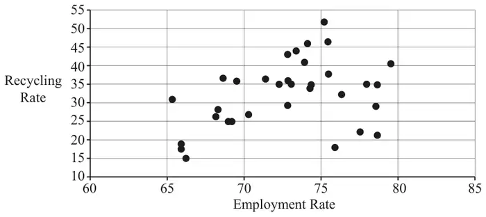
Fig. 13.1: scatter diagram of recycling rate (10 to 55) against employment rate (60 to 85) for 33 regions, showing weak positive correlation — Fig. 13.1

The product moment correlation coefficient for this sample is 0.37154 and the associated \(p\)-value is 0.033.

Lee conducts a hypothesis test at the 5% level to test whether there is any evidence to suggest there is positive correlation between recycling rate and employment rate. He concludes that there is no evidence to suggest positive correlation because \(0.033 \approx 0\) and \(0.37154 > 0.05\).

(a) Explain whether Lee’s reasoning is correct. [2]

Fig. 13.2 shows a scatter diagram of recycling rate against median house price for a random sample of 33 regions.

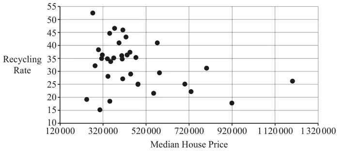
Fig. 13.2: scatter diagram of recycling rate against median house price (120 000 to 1 320 000) for 33 regions; most points lie between 250 000 and 550 000, with isolated points near 920 000 and 1 200 000 — Fig. 13.2

The product moment correlation coefficient for this sample is \(-0.33278\) and the associated \(p\)-value is 0.058.

Fig. 13.3 shows summary statistics for the median house prices for the data in this sample.

Statistics
n	33
Mean	465467.9697
σ	201236.1345
s	204356.2606
Σx	15360443
Σx²	8486161617387
Min	243500
Q1	342500
Median	410000
Q3	521000
Max	1200000

Fig. 13.3

(b) Use the information in Fig. 13.3 and Fig. 13.2 to show that there are at least two outliers. [2]

the product moment correlation coefficient between recycling rate and median house price,
the \(p\)-value associated with this correlation coefficient,

in each case explaining your answer. [2]

All 33 items in the sample are areas in London. A student suggests that it is very unlikely that only areas in London would be selected in a random sample.

(d) Use your knowledge of the pre-release material to explain whether you think the student’s suggestion is reasonable. [1]

Mark scheme (a)

Scheme	Marks	AO
Lee is wrong because he should make the comparison of 0.033 with 0.05	B1	2.2a
he should make the comparison of 0.37154 with 0	B1	2.2b
	[2]

Notes

B1: allow he should have compared \(r\) with the critical value

if B0B0 SC1 for Lee has confused \(r\) with \(p\) or for 0.37154 suggests positive correlation

Mark scheme (b)

Scheme	Marks	AO
\(465467 + 2 \times 204356\)	M1	2.1
awrt 874180 (or 867940 from use of 201236) from scatter diagram the outliers are approximately 920 000, 1 200 000	A1	2.2b
	[2]

Notes

M1: condone use of 201236 instead of 204356;
ignore work relating to lower tail
or \(521000 + 1.5 \times (521000 - 342500)\)

A1: numerical values must be mentioned
or 788750 in which case accept two or three outliers identified extra one is approximately 800 000
(corrected from the printed mark scheme: “867940 from use of 210236” is printed; 867940 comes from 201236)

Mark scheme (c)

Scheme	Marks	AO
the pmcc would (probably) be closer to 0 because the scatter is less well modelled by a straight line	B1	2.2b
the \(p\)-value would increase because a value which is closer to 0 is more likely assuming there is no correlation	B1	2.2b
	[2]

Notes

if B0B0 allow SC1 for \(r\) closer to 0 and \(p\)-value larger