
June 2019 Paper 2 Q11
11 A trainer was asked to give a lecture on population profiles in different Local Authorities (LAs) in the UK. Using data from the 2011 census, he created the following scatter diagram for 17 selected LAs.
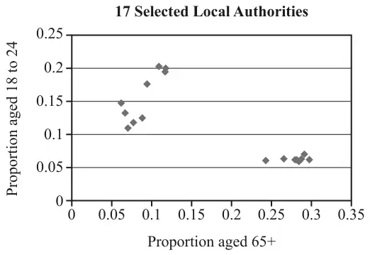
He selected the 17 LAs using the following method. The proportions of people aged 18 to 24 and aged 65+ in any Local Authority are denoted by \(P_{\text{young}}\) and \(P_{\text{senior}}\) respectively. The trainer used a spreadsheet to calculate the value of \(k = \dfrac{P_{\text{young}}}{P_{\text{senior}}}\) for each of the 348 LAs in the UK. He then used specific ranges of values of \(k\) to select the 17 LAs.
\(\mathrm{H}_0\): There is no linear correlation in the population between \(P_{\text{young}}\) and \(P_{\text{senior}}\).
\(\mathrm{H}_1\): There is negative linear correlation in the population between \(P_{\text{young}}\) and \(P_{\text{senior}}\).
He found that the value of Pearson’s product-moment correlation coefficient for the 17 LAs is \(-0.797\), correct to 3 significant figures.
The trainer concluded that there is evidence of negative linear correlation between \(P_{\text{young}}\) and \(P_{\text{senior}}\) in the population.
Suggest a reason why the diagram might be of particular interest to these people. [1]
Critical values of Pearson’s product-moment correlation coefficient
| 1-tail test | 5% | 2.5% | 1% | 0.5% |
|---|---|---|---|---|
| 2-tail test | 10% | 5% | 2% | 1% |
| \(n\) | ||||
| 1 | - | - | - | - |
| 2 | - | - | - | - |
| 3 | 0.9877 | 0.9969 | 0.9995 | 0.9999 |
| 4 | 0.9000 | 0.9500 | 0.9800 | 0.9900 |
| 5 | 0.8054 | 0.8783 | 0.9343 | 0.9587 |
| 6 | 0.7293 | 0.8114 | 0.8822 | 0.9172 |
| 7 | 0.6694 | 0.7545 | 0.8329 | 0.8745 |
| 8 | 0.6215 | 0.7067 | 0.7887 | 0.8343 |
| 9 | 0.5822 | 0.6664 | 0.7498 | 0.7977 |
| 10 | 0.5494 | 0.6319 | 0.7155 | 0.7646 |
| 11 | 0.5214 | 0.6021 | 0.6851 | 0.7348 |
| 12 | 0.4973 | 0.5760 | 0.6581 | 0.7079 |
| 13 | 0.4762 | 0.5529 | 0.6339 | 0.6835 |
| 14 | 0.4575 | 0.5324 | 0.6120 | 0.6614 |
| 15 | 0.4409 | 0.5140 | 0.5923 | 0.6411 |
| 16 | 0.4259 | 0.4973 | 0.5742 | 0.6226 |
| 17 | 0.4124 | 0.4821 | 0.5577 | 0.6055 |
| 18 | 0.4000 | 0.4683 | 0.5425 | 0.5897 |
| 19 | 0.3887 | 0.4555 | 0.5285 | 0.5751 |
| 20 | 0.3783 | 0.4438 | 0.5155 | 0.5614 |
| 21 | 0.3687 | 0.4329 | 0.5034 | 0.5487 |
| 22 | 0.3598 | 0.4227 | 0.4921 | 0.5368 |
| 23 | 0.3515 | 0.4132 | 0.4815 | 0.5256 |
| 24 | 0.3438 | 0.4044 | 0.4716 | 0.5151 |
| 25 | 0.3365 | 0.3961 | 0.4622 | 0.5052 |
| 26 | 0.3297 | 0.3882 | 0.4534 | 0.4958 |
| 27 | 0.3233 | 0.3809 | 0.4451 | 0.4869 |
| 28 | 0.3172 | 0.3739 | 0.4372 | 0.4785 |
| 29 | 0.3115 | 0.3673 | 0.4297 | 0.4705 |
| 30 | 0.3061 | 0.3610 | 0.4226 | 0.4629 |
| Scheme | Marks | AO |
|---|---|---|
| \(k \gt 1.4\) (allow \(k \gt 1.1\) to 1.6) \(k \lt 0.25\) (allow \(k \lt 0.2\) to 0.3) | B1 B1 | 2.2b 2.2b |
| or \(1.4 \lt k \lt \ldots\ldots\) B1 \(\ldots\ldots \lt k \lt 0.25\) (ranges as above) B1 | ||
| [2] |
Notes
Allow \(\geqslant\) and \(\leqslant\)
SC: \(0.25 \lt k \lt 1.4\): B1B0 (ranges as on left)
Allow "\(x\)"
| Scheme | Marks | AO |
|---|---|---|
| (i) \(0.797 \gt 0.5577\) or \(-0.797 \lt -0.5577\) or \(|-0.797| \gt 0.5577\) | B2 | 3.1b 3.2a |
| [2] | ||
| (ii) There are clusters (or groups etc.) | B1* | 2.3 |
| Apparent good correlation caused by clusters or Two clusters with no –ve corr'n within them or a comment similar to one of the above. AND Conclusion unreliable or Value of \(r\) is misleading oe | B1 dep B1* | 3.5b |
| [2] |
Notes
(b)(i) B2: \(0.797 \gt 0.6055\) or \(-0.797 \lt -0.6055\) B1
\(\pm 0.5577\) B1
Allow \(\geqslant\) or \(\leqslant\)
(b)(ii)
or Not bivariate normal distribution B1
so use of tables for \(r\) not valid B1
NOT Too scattered
Not represent whole pop
Small sample
Clusters not on reg line B1B0
| Scheme | Marks | AO |
|---|---|---|
| High prop of 65+ or Low prop of 18-24 Prop of young very similar, or \(\approx 0.06\) Proportion of senior to young is high | B1 | 2.2b |
| [1] |
Notes
B1: If consider only one age-group, must be proportion not number
If consider both age-groups, allow eg
Higher number of seniors than young or
Many seniors, few young
NOT:
Similar proportions of 65+
Population is elderly
| Scheme | Marks | AO |
|---|---|---|
| Top left points contain high prop of 18-24s. (So these LAs may be areas where there are universities or where they can recruit) | B1 | 2.2b |
| [1] |
Notes
B1: Shows places where large nos of 18-24s
Shows where to focus recruiting.
So universities can recruit.
18-24s are their target group.
No need to specify "Top left group"
Allow "students" or "young" instead of "18-24s"
Any implication that diagram enables you to see information about location of young people