June 2022 Paper 2 Q9

OCR ACurrent spec14 marksData Processing Normal Distribution

9 The heights, in centimetres, of a random sample of 150 plants of a certain variety were measured. The results are summarised in the histogram.

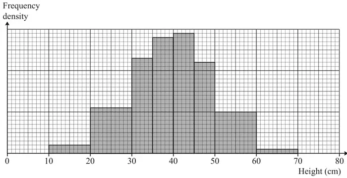
Histogram of frequency density against height in cm from 0 to 80, with bars for 10 to 20, 20 to 30, 30 to 35, 35 to 40, 40 to 45, 45 to 50, 50 to 60 and 60 to 70; the tallest bars are 35 to 40 and 40 to 45

One of the 150 plants is chosen at random, and its height, \(X\) cm, is noted.

(a) Show that \(\mathrm{P}(20 \lt X \lt 30) = 0.147\), correct to 3 significant figures. [2]

Sam suggests that the distribution of \(X\) can be well modelled by the distribution \(\mathrm{N}(40, 100)\).

(b)

(i) Give a brief justification for the use of the normal distribution in this context. [1]

(ii) Give a brief justification for the choice of the parameter values 40 and 100. [2]

Nina suggests a different model. She uses the midpoints of the classes to calculate estimates, \(m\) and \(s\), for the mean and standard deviation respectively, in centimetres, of the 150 heights. She then uses the distribution \(\mathrm{N}(m, s^2)\) as her model.

(d) Use Nina’s model to find \(\mathrm{P}(20 \lt X \lt 30)\). [4]

(e)

(i) Complete the table in the Printed Answer Booklet to show the probabilities obtained from Sam’s model and Nina’s model. [2]

\(x\)	< 20	20 to 30	30 to 35	35 to 40	40 to 45	45 to 50	50 to 60	> 60
Histogram	0.027	0.147	0.153	0.187	0.193	0.147	0.133	0.013
\(\mathrm{N}(40, 100)\)	0.023		0.150	0.191			0.136	0.023
\(\mathrm{N}(m, s^2)\)	0.030		0.153	0.189			0.130	0.023

(ii) By considering the different ranges of values of \(X\) given in the table, discuss how well the two models fit the original distribution. [2]

Mark scheme (a)

Scheme	Marks	AO
Area of 20-30 block ÷ total area	M1	1.2
\(= \dfrac{110}{750}\) or \(\dfrac{22}{150}\) or \(\dfrac{4.4}{30}\) \(= 0.147\) (3 sf) (AG)	A1	1.1
	[2]

Notes

M1: attempted, using any units, eg small squares or cm²

A1: Correct calculation seen and answer 0.147 seen
Not any method starting with 0.147, eg \(0.147 \times 150 = 22.05\)

Mark scheme (b)

Scheme	Marks	AO
(i) Roughly bell-shaped	B1	2.2b
	[1]
(ii) Roughly symmetrical about \(x = 40\), or area to left of 40 \(\approx\) area to right of 40 or the peak is at 40 or 40 is in the middle	B1	2.4
\(70 - 40 \approx 3\sigma\), hence \(\sigma \approx 10\) or most values within 20 of mean, so \(20 \approx 2\sigma\) or (Area within \(40 \pm 10\))/total eg 510/750 or \(102/150 = 0.68\) or \(\approx \frac{2}{3}\)	B1	3.3
	[2]

Notes

(b)(i)

B1: or Roughly symmetrical and peaks in middle or has one peak and tails off at each end, or drops off either side
All 3 of these must be seen (except “Bell-shaped” scores B1)
Not “Shape is like normal curve” Ignore all else

(b)(ii)

B1: or calculate mean and obtain \(\frac{5915}{150}\) or 39.4
Allow 40 has the highest frequency or frequency density
Ignore all else

B1: or calculate sd and obtain 10.3
Most data is within \(6\sigma\)
Must see correct fraction and \(\approx \frac{2}{3}\), or 68% or 0.68

Scheme	Marks	AO
0.136 (3 sf)	B1	1.1
	[1]

Mark scheme (d)

Scheme	Marks	AO
\(m = 39.4\) or \(\dfrac{5915}{150}\) or \(\dfrac{1183}{30}\),	B1	3.1a
\(s = 10.3\) (3 sf) or \(s^2 = 106\) (3 sf)	B1	1.1
0.150 or 0.151 or 0.152 (3 sf) Allow 0.15	B2	3.4 1.1
	[4]

Notes

B1: Allow \(39.1 \leqslant m \leqslant 39.7\) Ignore method BC

B1: Allow \(105.5 \leqslant s^2 \leqslant 108.5\) or \(10.27 \leqslant s \leqslant 10.42\) Ignore method
(Use of denominator \(n\) or \((n - 1)\) is OK for full marks)
OR if neither mark scored,
M1 for attempting find frequencies or areas (NOT heights) or at least five of these seen: 4, 22, 23, 28, 29, 22, 20, 2
or 20, 110, 115, 140, 145, 110, 100, 10

B2: cao Correct with unclear or no working; B1B1B1B1
or B1 for 0.145 to 0.158

NB No retrospective marks if 0.151 seen in table for (e)(i)

Mark scheme (e)

Scheme

Marks

(i)

\(x\)	< 20	20 to 30	30 to 35	35 to 40	40 to 45	45 to 50	50 to 60	> 60
Histogram	0.027	0.147	0.153	0.187	0.193	0.147	0.133	0.013
\(\mathrm{N}(40, 100)\)	0.023	0.136	0.150	0.191	0.191	0.150	0.136	0.023
\(\mathrm{N}(m, s^2)\)	0.030	0.151	0.153	0.189	0.183	0.142	0.130	0.023

(the values to be found are in bold)

B1
B1

1.1
3.4

[2]

(ii) Nina's model better fit for lower values of \(X\)
Nina's model better fit for any ranges < 40
Nina’s model less good fit for 40-45 (or >60)

3.5a

Sam's model better fit for higher values
Sam's model better fit for any ranges > 40
Sam’s model less good fit for 20-30 (or >60)

3.5a

[2]

Notes

(e)(i)

No FT

B1 for middle row correct \(\pm 0.001\) NB

B1 for bottom row correct \(\pm 0.003\) NB

(e)(ii)

Allow “more accurate” or “less accurate” or similar

BUT SC: “Both less good fit for >60” alone: B1 only
NOT “Both are fairly good fit” B0B0
Ignore all else NB No ft