
June 2018 Paper 2 Q14
14 The pre-release material includes data on unemployment rates in different countries. A sample from this material has been taken. All the countries in the sample are in Europe. The data have been grouped and are shown in Fig 14.1.
| Unemployment rate | 0– | 5– | 10– | 15– | 20– | 35–50 |
|---|---|---|---|---|---|---|
| Frequency | 15 | 21 | 5 | 5 | 2 | 2 |
Fig. 14.1
A cumulative frequency curve has been generated for the sample data using a spreadsheet. This is shown in Fig. 14.2.
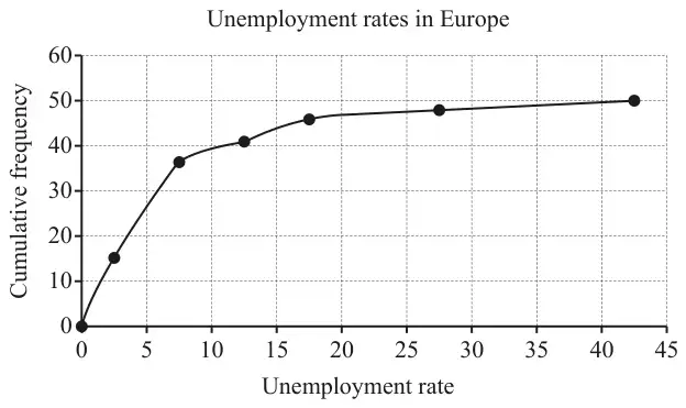
Hodge used Fig. 14.2 to estimate the median unemployment rate in Europe. He obtained the answer 5.0. The correct value for this sample is 6.9.
- Identify this error.
- State how this error affects Hodge’s estimate.
- Identify this factor.
- State how this factor affects Hodge’s estimate.
The scatter diagram shown in Fig. 14.3 shows the unemployment rate and life expectancy at birth for the 47 countries in the sample for which this information is available.
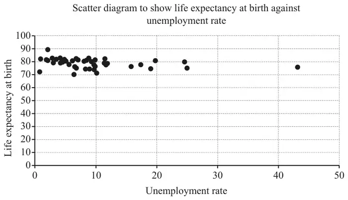
The product moment correlation coefficient for the 47 items in the sample is \(-0.2607\).
The \(p\)-value associated with \(r = -0.2607\) and \(n = 47\) is 0.0383.
Hodge uses the spreadsheet tools to obtain the equation of a line of best fit for this data.
| Scheme | Marks | AO |
|---|---|---|
| (A) the cumulative frequencies have been plotted against the mid-points of the class intervals, | B1 | 2.4 |
| mis-plotting [at centre of each class] reduces estimate (by 2.5) oe | B1 | 2.4 |
| [2] | ||
| (B) grouped data has been used | B1 | 2.4 |
| grouping has slightly reduced the error introduced by misplotting (because the error is less than 2.5) | B1 | 2.4 |
| [2] |
Notes
(B)
B1: or eg Hodge used the graph (instead of the raw data)
| Scheme | Marks | AO |
|---|---|---|
| percentage unemployment is often estimated oe | E1 | 2.4 |
| [1] |
Notes
E1: allow data (on percentage unemployment) is not available for all countries in Europe oe
| Scheme | Marks | AO |
|---|---|---|
| there are many other countries in the pre-release material; it is very unlikely that a random sample would only include European countries. | E1 | 2.4 |
| [1] |
| Scheme | Marks | AO |
|---|---|---|
| negative correlation / association (may be embedded) | B1 | 2.2b |
| comparison of \(p\)-value with 0.05 or 0.01 or other appropriate significance level and supporting comment | B1 | 2.2b |
| [2] |
Notes
if B0B0 allow SC2 for eg comment on no significant association justified by comparison of \(p\)-value with appropriate significance level (eg 0.025)
| Scheme | Marks | AO |
|---|---|---|
| (even though this is interpolation), the scatter / weak correlation / presence of an outlier would suggest that the use of a line of best fit is inappropriate | E1 | 2.2b |
| [1] |
Notes
E1: allow explanation based on the value for Kosovo being an outlier or on it lying in the (large) gap in the scatter