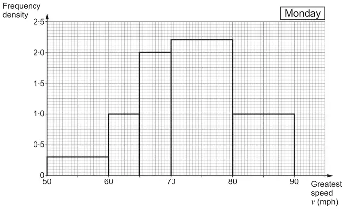
14. The histogram below represents the greatest speed, \(v\) mph, of a car when driven by 50 drivers on a section of racetrack on Monday.
(a) Calculate an estimate of the percentage of the 50 drivers who drove at a greatest speed of 75 mph or more on this section of racetrack. [3]
(b) Use the histogram to complete this cumulative frequency table. [2]
Greatest speed, \(v\) (mph)
\(v \leqslant 50\)
\(v \leqslant 60\)
\(v \leqslant 65\)
\(v \leqslant 70\)
\(v \leqslant 80\)
\(v \leqslant 90\)
Cumulative frequency
0
50
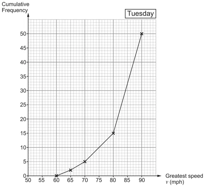
(c) The cumulative frequency diagram below represents the greatest speed, \(v\) mph, of the same car when driven by 50 different drivers on the same section of racetrack on Tuesday.
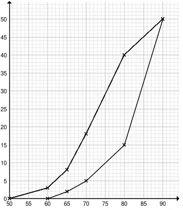
(i) On the grid above, draw the cumulative frequency diagram to represent the results of Monday’s drivers. [2]
(ii) On one of the days, many of the drivers were racing drivers.
On which day was this likely to be? Give numerical evidence and explain your decision. [2]
Mark scheme (a)
Scheme
Marks
Comments
21
B2
B1 for \(5 \times 2.2 + (1 \times)\ 10\)
42 (%)
B1
FT provided at least B1 awarded.
If no marks award SC1 for \(0.3 \times 10 + (1 \times)\ 5 + 2 \times 5 + 2.2 \times 10 + (1 \times)\ 10\)
Mark scheme (b)
Scheme
Marks
Comments
\(v\)
cf
\(v \leqslant 50\)
0
\(v \leqslant 60\)
3
\(v \leqslant 65\)
8
\(v \leqslant 70\)
18
\(v \leqslant 80\)
40
\(v \leqslant 90\)
50
B2
B1 FT for any 2 or 3 unshaded cells correct; FT ‘their 3’ + 5, ‘their 8’ + 10, ‘their 18’ + 22
Mark scheme (c)
Scheme
Marks
Comments
(c)(i) Correct cf diagram
B2
FT ‘their part (b)’ for B2 or B1 provided an attempt at cumulative frequency; may be a curve; lines need not be ruled
B1 FT for first 5 points plotted correctly but not joined or for at most 2 incorrectly plotted points which have been correctly joined
Tuesday indicated and valid interpretation using their numerical evidence e.g. ‘The median for Tuesday is greater, (so more had a higher greatest speed).’ or ‘The upper quartile for Tuesday is greater, so the top 25% of drivers drove more quickly.’
We'd like to use Google Analytics cookies to count visits and see which pages help most. They're optional, and the site works exactly the same either way. Privacy policy