
S4 June 2006 Q6
6.
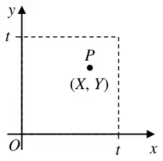
Figure 1 shows a square of side \(t\) and area \(t^2\) which lies in the first quadrant with one vertex at the origin. A point \(P\) with coordinates \((X, Y)\) is selected at random inside the square and the coordinates are used to estimate \(t^2\). It is assumed that \(X\) and \(Y\) are independent random variables each having a continuous uniform distribution over the interval \([0, t]\).
[You may assume that \(\mathrm{E}(X^nY^n) = \mathrm{E}(X^n)\mathrm{E}(Y^n)\), where \(n\) is a positive integer.]
The random variable \(S = kXY\), where \(k\) is a constant, is an unbiased estimator for \(t^2\).
The random variable \(U = q(X^2 + Y^2)\), where \(q\) is a constant, is also an unbiased estimator for \(t^2\).
The point \((2, 3)\) is selected from inside the square.
| Scheme | Marks |
|---|---|
| \(\mathrm{E}(X^n) = \displaystyle\int_0^t x^n \frac{1}{t}\,\mathrm{d}x = \left[\frac{x^{n+1}}{t(n+1)}\right]_0^t = \left(\frac{t^{n+1}}{t(n+1)} - 0\right) = \underline{\underline{\frac{t^n}{n+1}}}\) \(\displaystyle\int x^n \frac{1}{t}\) M1; \(\displaystyle\int_0^t \ldots \mathrm{d}x\) M1 | M1 M1 A1 cso |
| (3) |
| Scheme | Marks |
|---|---|
| \(\left(\mathrm{E}(X) = \dfrac{t}{2}\right) \qquad \underline{\mathrm{E}(S) = k\mathrm{E}(X)\mathrm{E}(Y)},\ = k \cdot \dfrac{t^2}{4}\) | M1, A1 |
| \(\mathrm{E}(S) = t^2 \Rightarrow \underline{k = 4}\) | A1 |
| (3) |
| Scheme | Marks |
|---|---|
| \(\mathrm{Var}(XY) = \mathrm{E}(X^2)\mathrm{E}(Y^2) - [\mathrm{E}(XY)]^2\) | M1 |
| \(= \dfrac{t^2}{3} \times \dfrac{t^2}{3} - \left(\dfrac{t^2}{4}\right)^2 = \left\{\dfrac{7t^4}{144}\right\}\) | M1 |
| \(\mathrm{Var}(S) = k^2\,\mathrm{Var}(XY) = 16 \times \dfrac{7t^4}{144} = \underline{\dfrac{7t^4}{9}}\) | A1 cso |
| (3) |
| Scheme | Marks |
|---|---|
| \(\mathrm{E}(U) = t^2 \Rightarrow 2\mathrm{E}(X^2)q = t^2,\ \Rightarrow 2\dfrac{t^2}{3}q = t^2,\ \Rightarrow \underline{q = \dfrac{3}{2}}\) | M1, M1, A1 cso |
| (3) |
| Scheme | Marks |
|---|---|
| \(\mathrm{Var}(U) = q^2[\mathrm{Var}(X^2) + \mathrm{Var}(Y^2)] = 2q^2\,\mathrm{Var}(X^2)\) | M1 |
| \(\mathrm{Var}(X^2) = \mathrm{E}(X^4) - [\mathrm{E}(X^2)]^2 = \dfrac{t^4}{5} - \left(\dfrac{t^2}{3}\right)^2 = \left(\dfrac{4}{45}t^4\right)\) | M1 |
| \(\mathrm{Var}(U) = 2 \times \dfrac{9}{4} \times \dfrac{4}{45}t^4 = \underline{\underline{\dfrac{2}{5}t^4}}\) | A1 |
| (3) |
| Scheme | Marks |
|---|---|
| \(\dfrac{2}{5} \lt \dfrac{7}{9} \quad \therefore U\) is better \(\because\) smaller variance | B1ft |
| (1) |
| Scheme | Marks |
|---|---|
| Using \(U\) estimate is: \(\dfrac{3}{2}(2^2 + 3^2) = \dfrac{3}{2} \times 13 = \underline{\underline{\dfrac{39}{2}}}\) or \(\underline{\underline{19.5}}\) | B1ft |
| (1) | |
| (17 marks) |