June 2018 Paper 3 Q4

EdexcelCurrent spec13 marksIncludes samplingData Processing

4. Charlie is studying the time it takes members of his company to travel to the office. He stands by the door to the office from 08 40 to 08 50 one morning and asks workers, as they arrive, how long their journey was.

(a) State the sampling method Charlie used. (1)

(b) State and briefly describe an alternative method of non-random sampling Charlie could have used to obtain a sample of 40 workers. (2)

Taruni decided to ask every member of the company the time, \(x\) minutes, it takes them to travel to the office.

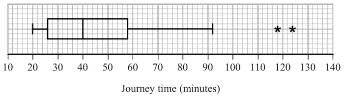
Taruni’s results are summarised by the box plot and summary statistics below.

box plot of journey time in minutes on a scale from 10 to 140: lower whisker at 20, lower quartile 26, median 40, upper quartile 58, upper whisker at 92, and two outliers marked with asterisks at about 118 and 124

\[n = 95 \qquad \sum x = 4133 \qquad \sum x^2 = 202\,294\]

(d) Write down the interquartile range for these data. (1)

(e) Calculate the mean and the standard deviation for these data. (3)

(f) State, giving a reason, whether you would recommend using the mean and standard deviation or the median and interquartile range to describe these data. (2)

Rana and David both work for the company and have both moved house since Taruni collected her data.

Rana’s journey to work has changed from 75 minutes to 35 minutes and David’s journey to work has changed from 60 minutes to 33 minutes.

Taruni drew her box plot again and only had to change two values.

(g) Explain which two values Taruni must have changed and whether each of these values has increased or decreased. (3)

Scheme	Marks	AO
Convenience or opportunity [sampling]	B1	1.2
	(1)

Mark scheme (b)

Scheme	Marks	AO
Quota [sampling]	B1	1.1a
e.g. Take 4 people every 10 minutes	B1	1.1b
	(2)

Notes

1^st B1 for quota (sampling) mentioned (“Stratified” or “systematic” or “random” are B0B0)

2^nd B1 for a description of how such a system might work, requires suitable strata or categories
e.g. time slots, departments, gender, age groups, distance travelled etc
Suggestion of randomness is B0

Scheme	Marks	AO
Census	B1	1.2
	(1)

Scheme	Marks	AO
\([58 - 26 =]\ \underline{32}\) (min)	B1	1.1b
	(1)

Mark scheme (e)

Scheme	Marks	AO
\(\mu = \dfrac{4133}{95} = 43.505263\ldots\) awrt 43.5 (min)	B1	1.1b
\(\sigma_x = \sqrt{\dfrac{202\,294}{95} - \mu^2} = \sqrt{236.7026\ldots}\)	M1	1.1b
\(= 15.385\ldots\) awrt 15.4 (min)	A1	1.1b
	(3)

Notes

B1 for a correct mean (awrt 43.5)

M1 for a correct expression for the sd (including \(\sqrt{\ }\)) ft their mean

A1 for awrt 15.4 (Allow \(s = 15.4667\ldots\) awrt 15.5)

Mark scheme (f)

Scheme	Marks	AO
There are outliers in the data (or data is skew) which will affect mean and sd	B1	2.4
Therefore use median and IQR	dB1	2.4
	(2)

Notes

1^st B1 for acknowledging outliers or skewness are a problem for mean and sd
“extreme values”/“anomalies” OK May be implied by saying median and IQR not affected by..
We need to see mention of “outliers”, “skewness” and the problem so “data is skewed so use median and IQR” is B0 unless mention that they are not affected by extreme values or mean and standard deviation can be “inflated” by the positive skew etc

2^nd dB1 dep on 1^st B1 for therefore choosing median and IQR

Mark scheme (g)

Scheme	Marks	AO
Value of 20, LQ at 26 and outliers will not change or state that median and upper quartile are the values that do change	B1	1.1b
More values now below 40 than above so \(Q_2\) or \(Q_3\) will change and be lower	M1	2.1
Both \(Q_2\) and \(Q_3\) will be lower	A1	2.4
	(3)
	(13 marks)

Notes

B1 for identifying 2 of these 3 groups of unchanged values or stating only \(Q_2\) and \(Q_3\) change

M1 for explaining that median or UQ should be lower.
E.g. the 2 values have moved to below 40 (or 58) and therefore more than 50% below 40 or (more than 75% below 58) or an argument to show that the other 3 values are the same. (o.e.)
Allow arrows on box plot provided statement in words about increased % below 40 or 58 etc

A1 for stating median and UQ are both lower with clear evidence of M1 scored

[If lots of values on 40 then median might not change but, since two values do change then UQ would change. If this meant that 92 became an outlier then we would have a new value for upper whisker and an extra outlier so effectively 3 values are altered. So median changes]